5. More Info: Climate and Model Data Access

Tutorials at the 2026 paleoCAMP | June 15–June 29, 2026

Jiang Zhu
jiangzhu@ucar.edu
Climate & Global Dynamics Laboratory
NSF National Center for Atmospheric Research

---

More information and examples to demonstrate data access and analysis

• Guidance on using climate data

• Access Earth System Model output

• NCAR JupyterHub is your one-stop shop for data access and analysis!

  • Example 1: Access ERA5 Reanalysis on NSF NCAR’s Research Data Archive

  • Example 2: Access CESM output on NCAR’s Campaign Storage and perform model-data comparison

Time to learn: 15 minutes

---

Guidance on using climate data

• NCAR Climate Data Guide: Key strengths, Key limitations, Expert User Guidance, etc.

  • Atmospheric Reanalysis: Overview & Comparison Tables

  • Paleoclimate (You could contribute!)

  • …

---

Access ESM output

• Earth System Grid Federation (ESGF), e.g., the LLNL Node

• NSF NCAR Geoscience Data Exchange: e.g., ERA5 Reanalysis (1.77 PB!) and iTRACE

• CESM Paleoclimate Working Group webpage

• Other portals, such as the DeepMIP Model Database

---

NCAR JupyterHub is your one-stop shop for data access and analysis!

• Multiple PB of CESM Paleoclimate simulation data

• Other CESM simulation data

• Preinstalled Python environment

• Available recipes and examples

  • GeoCAT-examples

  • GDEX-examples)

Note: variable names may be different depending on the portals (IPCC Standard; CESM Standard)

---

Load Python packages

import os
import glob
from datetime import timedelta

import xarray as xr
import numpy as np
import pandas as pd

import matplotlib as mpl
import matplotlib.pyplot as plt
import cartopy.crs as ccrs
from cartopy.util import add_cyclic_point

# xesmf is used for regridding ocean output
import xesmf

import warnings
warnings.filterwarnings("ignore")

---

Example 1: Access ERA5 Reanalysis data on NSF NCAR’s Geoscience Data Exchange (GDEX)

• Browse the GDEX website and figure out the file structure

  • Search era5

  • Click the Monthly Mean product (d633001)

  • Click the tab DATA ACCESS

  • Total precipitation is in ERA5 monthly mean atmospheric surface forecast (accumulated) [netCDF4]

  • Click GLADE File Listing to see all the files stored on the NCAR Campaign Storage

• Or, you could follow the GDEX usage examples to use intake-esm

data_dir = '/glade/campaign/collections/gdex/data/d633001/e5.moda.fc.sfc.accumu/'

files_tp = glob.glob(data_dir + '*/*_tp.*.nc')
print(*sorted(files_tp), sep='\n')

/glade/campaign/collections/gdex/data/d633001/e5.moda.fc.sfc.accumu/1979/e5.moda.fc.sfc.accumu.128_228_tp.ll025sc.1979010100_1979120100.nc
/glade/campaign/collections/gdex/data/d633001/e5.moda.fc.sfc.accumu/1980/e5.moda.fc.sfc.accumu.128_228_tp.ll025sc.1980010100_1980120100.nc
/glade/campaign/collections/gdex/data/d633001/e5.moda.fc.sfc.accumu/1981/e5.moda.fc.sfc.accumu.128_228_tp.ll025sc.1981010100_1981120100.nc
/glade/campaign/collections/gdex/data/d633001/e5.moda.fc.sfc.accumu/1982/e5.moda.fc.sfc.accumu.128_228_tp.ll025sc.1982010100_1982120100.nc
/glade/campaign/collections/gdex/data/d633001/e5.moda.fc.sfc.accumu/1983/e5.moda.fc.sfc.accumu.128_228_tp.ll025sc.1983010100_1983120100.nc
/glade/campaign/collections/gdex/data/d633001/e5.moda.fc.sfc.accumu/1984/e5.moda.fc.sfc.accumu.128_228_tp.ll025sc.1984010100_1984120100.nc
/glade/campaign/collections/gdex/data/d633001/e5.moda.fc.sfc.accumu/1985/e5.moda.fc.sfc.accumu.128_228_tp.ll025sc.1985010100_1985120100.nc
/glade/campaign/collections/gdex/data/d633001/e5.moda.fc.sfc.accumu/1986/e5.moda.fc.sfc.accumu.128_228_tp.ll025sc.1986010100_1986120100.nc
/glade/campaign/collections/gdex/data/d633001/e5.moda.fc.sfc.accumu/1987/e5.moda.fc.sfc.accumu.128_228_tp.ll025sc.1987010100_1987120100.nc
/glade/campaign/collections/gdex/data/d633001/e5.moda.fc.sfc.accumu/1988/e5.moda.fc.sfc.accumu.128_228_tp.ll025sc.1988010100_1988120100.nc
/glade/campaign/collections/gdex/data/d633001/e5.moda.fc.sfc.accumu/1989/e5.moda.fc.sfc.accumu.128_228_tp.ll025sc.1989010100_1989120100.nc
/glade/campaign/collections/gdex/data/d633001/e5.moda.fc.sfc.accumu/1990/e5.moda.fc.sfc.accumu.128_228_tp.ll025sc.1990010100_1990120100.nc
/glade/campaign/collections/gdex/data/d633001/e5.moda.fc.sfc.accumu/1991/e5.moda.fc.sfc.accumu.128_228_tp.ll025sc.1991010100_1991120100.nc
/glade/campaign/collections/gdex/data/d633001/e5.moda.fc.sfc.accumu/1992/e5.moda.fc.sfc.accumu.128_228_tp.ll025sc.1992010100_1992120100.nc
/glade/campaign/collections/gdex/data/d633001/e5.moda.fc.sfc.accumu/1993/e5.moda.fc.sfc.accumu.128_228_tp.ll025sc.1993010100_1993120100.nc
/glade/campaign/collections/gdex/data/d633001/e5.moda.fc.sfc.accumu/1994/e5.moda.fc.sfc.accumu.128_228_tp.ll025sc.1994010100_1994120100.nc
/glade/campaign/collections/gdex/data/d633001/e5.moda.fc.sfc.accumu/1995/e5.moda.fc.sfc.accumu.128_228_tp.ll025sc.1995010100_1995120100.nc
/glade/campaign/collections/gdex/data/d633001/e5.moda.fc.sfc.accumu/1996/e5.moda.fc.sfc.accumu.128_228_tp.ll025sc.1996010100_1996120100.nc
/glade/campaign/collections/gdex/data/d633001/e5.moda.fc.sfc.accumu/1997/e5.moda.fc.sfc.accumu.128_228_tp.ll025sc.1997010100_1997120100.nc
/glade/campaign/collections/gdex/data/d633001/e5.moda.fc.sfc.accumu/1998/e5.moda.fc.sfc.accumu.128_228_tp.ll025sc.1998010100_1998120100.nc
/glade/campaign/collections/gdex/data/d633001/e5.moda.fc.sfc.accumu/1999/e5.moda.fc.sfc.accumu.128_228_tp.ll025sc.1999010100_1999120100.nc
/glade/campaign/collections/gdex/data/d633001/e5.moda.fc.sfc.accumu/2000/e5.moda.fc.sfc.accumu.128_228_tp.ll025sc.2000010100_2000120100.nc
/glade/campaign/collections/gdex/data/d633001/e5.moda.fc.sfc.accumu/2001/e5.moda.fc.sfc.accumu.128_228_tp.ll025sc.2001010100_2001120100.nc
/glade/campaign/collections/gdex/data/d633001/e5.moda.fc.sfc.accumu/2002/e5.moda.fc.sfc.accumu.128_228_tp.ll025sc.2002010100_2002120100.nc
/glade/campaign/collections/gdex/data/d633001/e5.moda.fc.sfc.accumu/2003/e5.moda.fc.sfc.accumu.128_228_tp.ll025sc.2003010100_2003120100.nc
/glade/campaign/collections/gdex/data/d633001/e5.moda.fc.sfc.accumu/2004/e5.moda.fc.sfc.accumu.128_228_tp.ll025sc.2004010100_2004120100.nc
/glade/campaign/collections/gdex/data/d633001/e5.moda.fc.sfc.accumu/2005/e5.moda.fc.sfc.accumu.128_228_tp.ll025sc.2005010100_2005120100.nc
/glade/campaign/collections/gdex/data/d633001/e5.moda.fc.sfc.accumu/2006/e5.moda.fc.sfc.accumu.128_228_tp.ll025sc.2006010100_2006120100.nc
/glade/campaign/collections/gdex/data/d633001/e5.moda.fc.sfc.accumu/2007/e5.moda.fc.sfc.accumu.128_228_tp.ll025sc.2007010100_2007120100.nc
/glade/campaign/collections/gdex/data/d633001/e5.moda.fc.sfc.accumu/2008/e5.moda.fc.sfc.accumu.128_228_tp.ll025sc.2008010100_2008120100.nc
/glade/campaign/collections/gdex/data/d633001/e5.moda.fc.sfc.accumu/2009/e5.moda.fc.sfc.accumu.128_228_tp.ll025sc.2009010100_2009120100.nc
/glade/campaign/collections/gdex/data/d633001/e5.moda.fc.sfc.accumu/2010/e5.moda.fc.sfc.accumu.128_228_tp.ll025sc.2010010100_2010120100.nc
/glade/campaign/collections/gdex/data/d633001/e5.moda.fc.sfc.accumu/2011/e5.moda.fc.sfc.accumu.128_228_tp.ll025sc.2011010100_2011120100.nc
/glade/campaign/collections/gdex/data/d633001/e5.moda.fc.sfc.accumu/2012/e5.moda.fc.sfc.accumu.128_228_tp.ll025sc.2012010100_2012120100.nc
/glade/campaign/collections/gdex/data/d633001/e5.moda.fc.sfc.accumu/2013/e5.moda.fc.sfc.accumu.128_228_tp.ll025sc.2013010100_2013120100.nc
/glade/campaign/collections/gdex/data/d633001/e5.moda.fc.sfc.accumu/2014/e5.moda.fc.sfc.accumu.128_228_tp.ll025sc.2014010100_2014120100.nc
/glade/campaign/collections/gdex/data/d633001/e5.moda.fc.sfc.accumu/2015/e5.moda.fc.sfc.accumu.128_228_tp.ll025sc.2015010100_2015120100.nc
/glade/campaign/collections/gdex/data/d633001/e5.moda.fc.sfc.accumu/2016/e5.moda.fc.sfc.accumu.128_228_tp.ll025sc.2016010100_2016120100.nc
/glade/campaign/collections/gdex/data/d633001/e5.moda.fc.sfc.accumu/2017/e5.moda.fc.sfc.accumu.128_228_tp.ll025sc.2017010100_2017120100.nc
/glade/campaign/collections/gdex/data/d633001/e5.moda.fc.sfc.accumu/2018/e5.moda.fc.sfc.accumu.128_228_tp.ll025sc.2018010100_2018120100.nc
/glade/campaign/collections/gdex/data/d633001/e5.moda.fc.sfc.accumu/2019/e5.moda.fc.sfc.accumu.128_228_tp.ll025sc.2019010100_2019120100.nc
/glade/campaign/collections/gdex/data/d633001/e5.moda.fc.sfc.accumu/2020/e5.moda.fc.sfc.accumu.128_228_tp.ll025sc.2020010100_2020120100.nc
/glade/campaign/collections/gdex/data/d633001/e5.moda.fc.sfc.accumu/2021/e5.moda.fc.sfc.accumu.128_228_tp.ll025sc.2021010100_2021120100.nc
/glade/campaign/collections/gdex/data/d633001/e5.moda.fc.sfc.accumu/2022/e5.moda.fc.sfc.accumu.128_228_tp.ll025sc.2022010100_2022120100.nc

ds = xr.open_mfdataset(files_tp)
ds = ds.reindex(latitude=sorted(ds.latitude.values))
ds

<xarray.Dataset> Size: 2GB
Dimensions:    (latitude: 721, longitude: 1440, time: 528)
Coordinates:
  * latitude   (latitude) float64 6kB -90.0 -89.75 -89.5 ... 89.5 89.75 90.0
  * longitude  (longitude) float64 12kB 0.0 0.25 0.5 0.75 ... 359.2 359.5 359.8
  * time       (time) datetime64[ns] 4kB 1979-01-01 1979-02-01 ... 2022-12-01
Data variables:
    TP         (time, latitude, longitude) float32 2GB dask.array<chunksize=(3, 360, 776), meta=np.ndarray>
    utc_date   (time) int32 2kB dask.array<chunksize=(12,), meta=np.ndarray>
Attributes:
    DATA_SOURCE:          ECMWF: https://cds.climate.copernicus.eu, Copernicu...
    NETCDF_CONVERSION:    CISL RDA: Conversion from ECMWF GRIB 1 data to netC...
    NETCDF_VERSION:       4.6.1
    CONVERSION_PLATFORM:  Linux casper02 3.10.0-693.21.1.el7.x86_64 #1 SMP We...
    CONVERSION_DATE:      Mon Nov 11 08:45:33 MST 2019
    Conventions:          CF-1.6
    NETCDF_COMPRESSION:   NCO: Precision-preserving compression to netCDF4/HD...
    history:              Mon Nov 11 08:45:34 2019: ncks -4 --ppc default=7 e...
    NCO:                  netCDF Operators version 4.7.9 (Homepage = http://n...

xarray.Dataset

• Dimensions:
  • latitude: 721
  • longitude: 1440
  • time: 528
• Coordinates: (3)
  • latitude
    (latitude)
    float64
    -90.0 -89.75 -89.5 ... 89.75 90.0

    long_name :

    latitude

    short_name :

    lat

    units :

    degrees_north

    array([-90.  , -89.75, -89.5 , ...,  89.5 ,  89.75,  90.  ], shape=(721,))

  • longitude
    (longitude)
    float64
    0.0 0.25 0.5 ... 359.2 359.5 359.8

    long_name :

    longitude

    short_name :

    lon

    units :

    degrees_east

    array([0.0000e+00, 2.5000e-01, 5.0000e-01, ..., 3.5925e+02, 3.5950e+02,
           3.5975e+02], shape=(1440,))

  • time
    (time)
    datetime64[ns]
    1979-01-01 ... 2022-12-01

    long_name :

    time

    array(['1979-01-01T00:00:00.000000000', '1979-02-01T00:00:00.000000000',
           '1979-03-01T00:00:00.000000000', ..., '2022-10-01T00:00:00.000000000',
           '2022-11-01T00:00:00.000000000', '2022-12-01T00:00:00.000000000'],
          shape=(528,), dtype='datetime64[ns]')

• Data variables: (2)
  • TP
    (time, latitude, longitude)
    float32
    dask.array<chunksize=(3, 360, 776), meta=np.ndarray>

    long_name :

    Total precipitation

    short_name :

    tp

    units :

    m

    original_format :

    WMO GRIB 1 with ECMWF local table

    ecmwf_local_table :

    128

    ecmwf_parameter :

    228

    minimum_value :

    0.0

    maximum_value :

    0.11752701

    grid_specification :

    0.25 degree x 0.25 degree from 90N to 90S and 0E to 359.75E (721 x 1440 Latitude/Longitude)

    rda_dataset :

    ds633.1

    rda_dataset_url :

    https:/rda.ucar.edu/datasets/ds633.1/

    rda_dataset_doi :

    DOI: 10.5065/P8GT-0R61

    rda_dataset_group :

    ERA5 monthly mean atmospheric surface forecast (accumulated) [netCDF4]

    number_of_significant_digits :

    7

    Array Chunk Bytes 2.04 GiB 3.21 MiB Shape (528, 721, 1440) (3, 361, 776) Dask graph 704 chunks in 90 graph layers Data type float32 numpy.ndarray

  • utc_date
    (time)
    int32
    dask.array<chunksize=(12,), meta=np.ndarray>

    long_name :

    UTC date yyyy-mm-dd hh:00:00 as yyyymmddhh

    units :

    Gregorian_year month day hour

    Array Chunk Bytes 2.06 kiB 48 B Shape (528,) (12,) Dask graph 44 chunks in 89 graph layers Data type int32 numpy.ndarray

• Attributes: (9)

  DATA_SOURCE :

  ECMWF: https://cds.climate.copernicus.eu, Copernicus Climate Data Store

  NETCDF_CONVERSION :

  CISL RDA: Conversion from ECMWF GRIB 1 data to netCDF4.

  NETCDF_VERSION :

  4.6.1

  CONVERSION_PLATFORM :

  Linux casper02 3.10.0-693.21.1.el7.x86_64 #1 SMP Wed Mar 7 19:03:37 UTC 2018 x86_64 x86_64 x86_64 GNU/Linux

  CONVERSION_DATE :

  Mon Nov 11 08:45:33 MST 2019

  Conventions :

  CF-1.6

  NETCDF_COMPRESSION :

  NCO: Precision-preserving compression to netCDF4/HDF5 (see "history" and "NCO" global attributes below for specifics).

  history :

  Mon Nov 11 08:45:34 2019: ncks -4 --ppc default=7 e5.moda.fc.sfc.accumu.128_228_tp.ll025sc.1979010100_1979120100.unc.nc e5.moda.fc.sfc.accumu.128_228_tp.ll025sc.1979010100_1979120100.nc

  NCO :

  netCDF Operators version 4.7.9 (Homepage = http://nco.sf.net, Code = http://github.com/nco/nco)

Change the units from m per day to mm per day and make a plot

See here for clarification of units.

tp = ds.TP.mean('time') * 1000.0
tp = tp.compute()
tp

<xarray.DataArray 'TP' (latitude: 721, longitude: 1440)> Size: 4MB
array([[0.18871191, 0.18871191, 0.18871191, ..., 0.18871191, 0.18871191,
        0.18871191],
       [0.1763593 , 0.17630874, 0.17631234, ..., 0.17640808, 0.17640086,
        0.17640446],
       [0.17613353, 0.17612088, 0.17608838, ..., 0.17611367, 0.17612632,
        0.17613533],
       ...,
       [0.6987416 , 0.69886446, 0.6989421 , ..., 0.6986495 , 0.69864047,
        0.69868386],
       [0.7080526 , 0.7081086 , 0.70814294, ..., 0.70803094, 0.7080472 ,
        0.70808154],
       [0.7012306 , 0.7012306 , 0.7012306 , ..., 0.7012306 , 0.7012306 ,
        0.7012306 ]], shape=(721, 1440), dtype=float32)
Coordinates:
  * latitude   (latitude) float64 6kB -90.0 -89.75 -89.5 ... 89.5 89.75 90.0
  * longitude  (longitude) float64 12kB 0.0 0.25 0.5 0.75 ... 359.2 359.5 359.8
Attributes: (12/14)
    long_name:                     Total precipitation
    short_name:                    tp
    units:                         m
    original_format:               WMO GRIB 1 with ECMWF local table
    ecmwf_local_table:             128
    ecmwf_parameter:               228
    ...                            ...
    grid_specification:            0.25 degree x 0.25 degree from 90N to 90S ...
    rda_dataset:                   ds633.1
    rda_dataset_url:               https:/rda.ucar.edu/datasets/ds633.1/
    rda_dataset_doi:               DOI: 10.5065/P8GT-0R61
    rda_dataset_group:             ERA5 monthly mean atmospheric surface fore...
    number_of_significant_digits:  7

xarray.DataArray

'TP'

• latitude: 721
• longitude: 1440

• 0.1887 0.1887 0.1887 0.1887 0.1887 ... 0.7012 0.7012 0.7012 0.7012

  array([[0.18871191, 0.18871191, 0.18871191, ..., 0.18871191, 0.18871191,
          0.18871191],
         [0.1763593 , 0.17630874, 0.17631234, ..., 0.17640808, 0.17640086,
          0.17640446],
         [0.17613353, 0.17612088, 0.17608838, ..., 0.17611367, 0.17612632,
          0.17613533],
         ...,
         [0.6987416 , 0.69886446, 0.6989421 , ..., 0.6986495 , 0.69864047,
          0.69868386],
         [0.7080526 , 0.7081086 , 0.70814294, ..., 0.70803094, 0.7080472 ,
          0.70808154],
         [0.7012306 , 0.7012306 , 0.7012306 , ..., 0.7012306 , 0.7012306 ,
          0.7012306 ]], shape=(721, 1440), dtype=float32)

• Coordinates: (2)
  • latitude
    (latitude)
    float64
    -90.0 -89.75 -89.5 ... 89.75 90.0

    long_name :

    latitude

    short_name :

    lat

    units :

    degrees_north

    array([-90.  , -89.75, -89.5 , ...,  89.5 ,  89.75,  90.  ], shape=(721,))

  • longitude
    (longitude)
    float64
    0.0 0.25 0.5 ... 359.2 359.5 359.8

    long_name :

    longitude

    short_name :

    lon

    units :

    degrees_east

    array([0.0000e+00, 2.5000e-01, 5.0000e-01, ..., 3.5925e+02, 3.5950e+02,
           3.5975e+02], shape=(1440,))

• Attributes: (14)

  long_name :

  Total precipitation

  short_name :

  tp

  units :

  m

  original_format :

  WMO GRIB 1 with ECMWF local table

  ecmwf_local_table :

  128

  ecmwf_parameter :

  228

  minimum_value :

  0.0

  maximum_value :

  0.11752701

  grid_specification :

  0.25 degree x 0.25 degree from 90N to 90S and 0E to 359.75E (721 x 1440 Latitude/Longitude)

  rda_dataset :

  ds633.1

  rda_dataset_url :

  https:/rda.ucar.edu/datasets/ds633.1/

  rda_dataset_doi :

  DOI: 10.5065/P8GT-0R61

  rda_dataset_group :

  ERA5 monthly mean atmospheric surface forecast (accumulated) [netCDF4]

  number_of_significant_digits :

  7

fig, ax = plt.subplots(
    nrows=1, ncols=1,
    figsize=(3, 1.5),
    subplot_kw={'projection': ccrs.Robinson(central_longitude=210)},
    constrained_layout=True)

# Plot model results using contourf
p0 = ax.contourf(tp.longitude, tp.latitude, tp,
                 levels=np.linspace(0, 16, 17),
                 cmap='YlGnBu', extend='both',
                 transform=ccrs.PlateCarree())
plt.colorbar(p0, ax=ax)
ax.coastlines(linewidth=0.5)
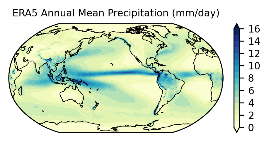
ax.set_title('ERA5 Annual Mean Precipitation (mm/day)', fontsize=8)

# plt.savefig('./precip_xy.era5.png', format='png', dpi=600, bbox_inches="tight")

Text(0.5, 1.0, 'ERA5 Annual Mean Precipitation (mm/day)')

---

Example 2: Access CESM paleoclimate output and perform model-data comparison on NCAR’s Campaign Storage

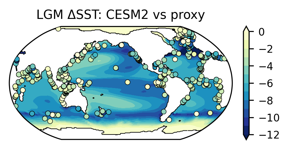
• We try to reproduce Figure 2a of Jiang’s paper to use the LGM ΔSST to assess CESM2’s climate sensitivity.

• Whole set of model output is shared at: /glade/campaign/cesm/community/palwg

• You can find additional simulation data here: /glade/campaign/cgd/ppc/jiangzhu

• Information of many CESM paleoclimate simulations is available on the Paleoclimate Working Group website

• As of now, prior knowledge of the experiments and file structure is needed. We hope to develop a Simulation Catalog for this!

!ls /glade/campaign/cesm/community/palwg/

ASD_paleoweather  iCESM1.2-DeglacialSlice  Past1000
cam6_paleo_ppe	  iTRACE		   Pliocene
CESM1-LME	  LastGlacialMaximum	   set_permission.csh
DECK		  LastInterglacial	   storage_use_policy.readme
Eocene		  Miocene		   TraCE
Holocene	  PaleoCalibr		   WisoMIP

!ls -l /glade/campaign/cesm/community/palwg/LastGlacialMaximum/CESM2
!ls /glade/campaign/cesm/community/palwg/LastGlacialMaximum/CESM2/b.e21.B1850CLM50SP.f09_g17.PI.01/ocn/proc/tseries/month_1/*.TEMP.*
!ls /glade/campaign/cesm/community/palwg/LastGlacialMaximum/CESM2/b.e21.B1850CLM50SP.f09_g17.21ka.01/ocn/proc/tseries/month_1/*.TEMP.*

total 3
drwxr-sr-x+ 7 jiangzhu cesm 4096 Aug  2  2024 b.e21.B1850CLM50SP.f09_g17.21ka.01
drwxr-sr-x+ 8 jiangzhu cesm 4096 Aug  2  2024 b.e21.B1850CLM50SP.f09_g17.PI.01
-rw-r--r--+ 1 jiangzhu cesm  413 Aug  2  2024 please_cite_zhu_etal_2021
/glade/campaign/cesm/community/palwg/LastGlacialMaximum/CESM2/b.e21.B1850CLM50SP.f09_g17.PI.01/ocn/proc/tseries/month_1/b.e21.B1850CLM50SP.f09_g17.PI.01.pop.h.TEMP.000101-010012.nc
/glade/campaign/cesm/community/palwg/LastGlacialMaximum/CESM2/b.e21.B1850CLM50SP.f09_g17.PI.01/ocn/proc/tseries/month_1/b.e21.B1850CLM50SP.f09_g17.PI.01.pop.h.TEMP.010101-020012.nc
/glade/campaign/cesm/community/palwg/LastGlacialMaximum/CESM2/b.e21.B1850CLM50SP.f09_g17.PI.01/ocn/proc/tseries/month_1/b.e21.B1850CLM50SP.f09_g17.PI.01.pop.h.TEMP.020101-030012.nc
/glade/campaign/cesm/community/palwg/LastGlacialMaximum/CESM2/b.e21.B1850CLM50SP.f09_g17.21ka.01/ocn/proc/tseries/month_1/b.e21.B1850CLM50SP.f09_g17.21ka.01.pop.h.TEMP.000101-010012.nc
/glade/campaign/cesm/community/palwg/LastGlacialMaximum/CESM2/b.e21.B1850CLM50SP.f09_g17.21ka.01/ocn/proc/tseries/month_1/b.e21.B1850CLM50SP.f09_g17.21ka.01.pop.h.TEMP.010101-020012.nc
/glade/campaign/cesm/community/palwg/LastGlacialMaximum/CESM2/b.e21.B1850CLM50SP.f09_g17.21ka.01/ocn/proc/tseries/month_1/b.e21.B1850CLM50SP.f09_g17.21ka.01.pop.h.TEMP.020101-030012.nc
/glade/campaign/cesm/community/palwg/LastGlacialMaximum/CESM2/b.e21.B1850CLM50SP.f09_g17.21ka.01/ocn/proc/tseries/month_1/b.e21.B1850CLM50SP.f09_g17.21ka.01.pop.h.TEMP.030101-040012.nc
/glade/campaign/cesm/community/palwg/LastGlacialMaximum/CESM2/b.e21.B1850CLM50SP.f09_g17.21ka.01/ocn/proc/tseries/month_1/b.e21.B1850CLM50SP.f09_g17.21ka.01.pop.h.TEMP.040101-050012.nc

campaign_dir = '/glade/campaign/cesm/community/palwg/LastGlacialMaximum/CESM2'
comp = 'ocn/proc/tseries/month_1'

Read preindustrial SST

case = 'b.e21.B1850CLM50SP.f09_g17.PI.01'
fname = 'b.e21.B1850CLM50SP.f09_g17.PI.01.pop.h.TEMP.020101-030012.nc'

file = os.path.join(campaign_dir, case, comp, fname)

# Open the file and select the last 10 years of data
ds_pre = xr.open_dataset(file).isel(time=slice(-120, None))
sst_pre = ds_pre.TEMP.isel(z_t=0).mean('time')
sst_pre

<xarray.DataArray 'TEMP' (nlat: 384, nlon: 320)> Size: 492kB
array([[       nan,        nan,        nan, ...,        nan,        nan,
               nan],
       [       nan,        nan,        nan, ...,        nan,        nan,
               nan],
       [-1.9042568, -1.9034731, -1.9024575, ...,        nan,        nan,
               nan],
       ...,
       [       nan,        nan,        nan, ...,        nan,        nan,
               nan],
       [       nan,        nan,        nan, ...,        nan,        nan,
               nan],
       [       nan,        nan,        nan, ...,        nan,        nan,
               nan]], shape=(384, 320), dtype=float32)
Coordinates:
    z_t      float32 4B 500.0
    ULONG    (nlat, nlon) float64 983kB ...
    ULAT     (nlat, nlon) float64 983kB ...
    TLONG    (nlat, nlon) float64 983kB ...
    TLAT     (nlat, nlon) float64 983kB ...
Dimensions without coordinates: nlat, nlon
Attributes:
    long_name:     Potential Temperature
    units:         degC
    grid_loc:      3111
    cell_methods:  time: mean

xarray.DataArray

'TEMP'

• nlat: 384
• nlon: 320

• nan nan nan nan nan nan nan nan ... nan nan nan nan nan nan nan nan

  array([[       nan,        nan,        nan, ...,        nan,        nan,
                 nan],
         [       nan,        nan,        nan, ...,        nan,        nan,
                 nan],
         [-1.9042568, -1.9034731, -1.9024575, ...,        nan,        nan,
                 nan],
         ...,
         [       nan,        nan,        nan, ...,        nan,        nan,
                 nan],
         [       nan,        nan,        nan, ...,        nan,        nan,
                 nan],
         [       nan,        nan,        nan, ...,        nan,        nan,
                 nan]], shape=(384, 320), dtype=float32)

• Coordinates: (5)
  • z_t
    ()
    float32
    500.0

    long_name :

    depth from surface to midpoint of layer

    units :

    centimeters

    positive :

    down

    valid_min :

    500.0

    valid_max :

    537500.0

    array(500., dtype=float32)

  • ULONG
    (nlat, nlon)
    float64
    ...

    long_name :

    array of u-grid longitudes

    units :

    degrees_east

    [122880 values with dtype=float64]

  • ULAT
    (nlat, nlon)
    float64
    ...

    long_name :

    array of u-grid latitudes

    units :

    degrees_north

    [122880 values with dtype=float64]

  • TLONG
    (nlat, nlon)
    float64
    ...

    long_name :

    array of t-grid longitudes

    units :

    degrees_east

    [122880 values with dtype=float64]

  • TLAT
    (nlat, nlon)
    float64
    ...

    long_name :

    array of t-grid latitudes

    units :

    degrees_north

    [122880 values with dtype=float64]

• Attributes: (4)

  long_name :

  Potential Temperature

  units :

  degC

  grid_loc :

  3111

  cell_methods :

  time: mean

Read LGM SST

case = 'b.e21.B1850CLM50SP.f09_g17.21ka.01'
fname = 'b.e21.B1850CLM50SP.f09_g17.21ka.01.pop.h.TEMP.040101-050012.nc'

file = os.path.join(campaign_dir, case, comp, fname)

# Open the file and select the last 10 years of data
ds_lgm = xr.open_dataset(file).isel(time=slice(-120, None))
sst_lgm = ds_lgm.TEMP.isel(z_t=0).mean('time')
sst_lgm

<xarray.DataArray 'TEMP' (nlat: 384, nlon: 320)> Size: 492kB
array([[nan, nan, nan, ..., nan, nan, nan],
       [nan, nan, nan, ..., nan, nan, nan],
       [nan, nan, nan, ..., nan, nan, nan],
       ...,
       [nan, nan, nan, ..., nan, nan, nan],
       [nan, nan, nan, ..., nan, nan, nan],
       [nan, nan, nan, ..., nan, nan, nan]],
      shape=(384, 320), dtype=float32)
Coordinates:
    z_t      float32 4B 500.0
    ULONG    (nlat, nlon) float64 983kB ...
    ULAT     (nlat, nlon) float64 983kB ...
    TLONG    (nlat, nlon) float64 983kB ...
    TLAT     (nlat, nlon) float64 983kB ...
Dimensions without coordinates: nlat, nlon
Attributes:
    long_name:     Potential Temperature
    units:         degC
    grid_loc:      3111
    cell_methods:  time: mean

xarray.DataArray

'TEMP'

• nlat: 384
• nlon: 320

• nan nan nan nan nan nan nan nan ... nan nan nan nan nan nan nan nan

  array([[nan, nan, nan, ..., nan, nan, nan],
         [nan, nan, nan, ..., nan, nan, nan],
         [nan, nan, nan, ..., nan, nan, nan],
         ...,
         [nan, nan, nan, ..., nan, nan, nan],
         [nan, nan, nan, ..., nan, nan, nan],
         [nan, nan, nan, ..., nan, nan, nan]],
        shape=(384, 320), dtype=float32)

• Coordinates: (5)
  • z_t
    ()
    float32
    500.0

    long_name :

    depth from surface to midpoint of layer

    units :

    centimeters

    positive :

    down

    valid_min :

    500.0

    valid_max :

    537500.0

    array(500., dtype=float32)

  • ULONG
    (nlat, nlon)
    float64
    ...

    long_name :

    array of u-grid longitudes

    units :

    degrees_east

    [122880 values with dtype=float64]

  • ULAT
    (nlat, nlon)
    float64
    ...

    long_name :

    array of u-grid latitudes

    units :

    degrees_north

    [122880 values with dtype=float64]

  • TLONG
    (nlat, nlon)
    float64
    ...

    long_name :

    array of t-grid longitudes

    units :

    degrees_east

    [122880 values with dtype=float64]

  • TLAT
    (nlat, nlon)
    float64
    ...

    long_name :

    array of t-grid latitudes

    units :

    degrees_north

    [122880 values with dtype=float64]

• Attributes: (4)

  long_name :

  Potential Temperature

  units :

  degC

  grid_loc :

  3111

  cell_methods :

  time: mean

Regrid into the 1° × 1° grid using xesmf

%%time

ds_pre['lat'] = ds_pre.TLAT
ds_pre['lon'] = ds_pre.TLONG

regridder = xesmf.Regridder(
    ds_in=ds_pre,
    ds_out=xesmf.util.grid_global(1, 1, cf=True, lon1=360),
    method='bilinear',
    periodic=True)

dsst_1x1 = regridder(sst_lgm - sst_pre)
dsst_1x1

CPU times: user 5.43 s, sys: 398 ms, total: 5.82 s
Wall time: 13 s

<xarray.DataArray (lat: 180, lon: 360)> Size: 259kB
array([[        nan,         nan,         nan, ...,         nan,
                nan,         nan],
       [        nan,         nan,         nan, ...,         nan,
                nan,         nan],
       [        nan,         nan,         nan, ...,         nan,
                nan,         nan],
       ...,
       [-0.17081444, -0.17075008, -0.17069343, ..., -0.17104828,
        -0.17096627, -0.1708865 ],
       [-0.178788  , -0.17878205, -0.17877994, ..., -0.17882909,
        -0.17881154, -0.17879783],
       [-0.18547155, -0.18547687, -0.18548317, ..., -0.18546143,
        -0.18546383, -0.1854672 ]], shape=(180, 360), dtype=float32)
Coordinates:
  * lat      (lat) float64 1kB -89.5 -88.5 -87.5 -86.5 ... 86.5 87.5 88.5 89.5
  * lon      (lon) float64 3kB 0.5 1.5 2.5 3.5 4.5 ... 356.5 357.5 358.5 359.5
    z_t      float32 4B 500.0
Attributes:
    regrid_method:  bilinear

xarray.DataArray

• lat: 180
• lon: 360

• nan nan nan nan nan nan ... -0.1855 -0.1855 -0.1855 -0.1855 -0.1855

  array([[        nan,         nan,         nan, ...,         nan,
                  nan,         nan],
         [        nan,         nan,         nan, ...,         nan,
                  nan,         nan],
         [        nan,         nan,         nan, ...,         nan,
                  nan,         nan],
         ...,
         [-0.17081444, -0.17075008, -0.17069343, ..., -0.17104828,
          -0.17096627, -0.1708865 ],
         [-0.178788  , -0.17878205, -0.17877994, ..., -0.17882909,
          -0.17881154, -0.17879783],
         [-0.18547155, -0.18547687, -0.18548317, ..., -0.18546143,
          -0.18546383, -0.1854672 ]], shape=(180, 360), dtype=float32)

• Coordinates: (3)
  • lat
    (lat)
    float64
    -89.5 -88.5 -87.5 ... 88.5 89.5

    bounds :

    lat_bounds

    standard_name :

    latitude

    units :

    degrees_north

    array([-89.5, -88.5, -87.5, -86.5, -85.5, -84.5, -83.5, -82.5, -81.5, -80.5,
           -79.5, -78.5, -77.5, -76.5, -75.5, -74.5, -73.5, -72.5, -71.5, -70.5,
           -69.5, -68.5, -67.5, -66.5, -65.5, -64.5, -63.5, -62.5, -61.5, -60.5,
           -59.5, -58.5, -57.5, -56.5, -55.5, -54.5, -53.5, -52.5, -51.5, -50.5,
           -49.5, -48.5, -47.5, -46.5, -45.5, -44.5, -43.5, -42.5, -41.5, -40.5,
           -39.5, -38.5, -37.5, -36.5, -35.5, -34.5, -33.5, -32.5, -31.5, -30.5,
           -29.5, -28.5, -27.5, -26.5, -25.5, -24.5, -23.5, -22.5, -21.5, -20.5,
           -19.5, -18.5, -17.5, -16.5, -15.5, -14.5, -13.5, -12.5, -11.5, -10.5,
            -9.5,  -8.5,  -7.5,  -6.5,  -5.5,  -4.5,  -3.5,  -2.5,  -1.5,  -0.5,
             0.5,   1.5,   2.5,   3.5,   4.5,   5.5,   6.5,   7.5,   8.5,   9.5,
            10.5,  11.5,  12.5,  13.5,  14.5,  15.5,  16.5,  17.5,  18.5,  19.5,
            20.5,  21.5,  22.5,  23.5,  24.5,  25.5,  26.5,  27.5,  28.5,  29.5,
            30.5,  31.5,  32.5,  33.5,  34.5,  35.5,  36.5,  37.5,  38.5,  39.5,
            40.5,  41.5,  42.5,  43.5,  44.5,  45.5,  46.5,  47.5,  48.5,  49.5,
            50.5,  51.5,  52.5,  53.5,  54.5,  55.5,  56.5,  57.5,  58.5,  59.5,
            60.5,  61.5,  62.5,  63.5,  64.5,  65.5,  66.5,  67.5,  68.5,  69.5,
            70.5,  71.5,  72.5,  73.5,  74.5,  75.5,  76.5,  77.5,  78.5,  79.5,
            80.5,  81.5,  82.5,  83.5,  84.5,  85.5,  86.5,  87.5,  88.5,  89.5])

  • lon
    (lon)
    float64
    0.5 1.5 2.5 ... 357.5 358.5 359.5

    bounds :

    lon_bounds

    standard_name :

    longitude

    units :

    degrees_east

    array([  0.5,   1.5,   2.5, ..., 357.5, 358.5, 359.5], shape=(360,))

  • z_t
    ()
    float32
    500.0

    array(500., dtype=float32)

• Attributes: (1)

  regrid_method :

  bilinear

Read proxy ΔSST in csv from Jess’s github

url = 'https://raw.githubusercontent.com/jesstierney/lgmDA/master/proxyData/Tierney2020_ProxyDataPaired.csv'
proxy_dsst = pd.read_csv(url)
proxy_dsst.head()

	Latitude	Longitude	Lower2s	Median	Upper2s	ProxyType	Species
0	-55.0	73.3	-2.927296	-1.379339	0.302709	delo	pachy
1	-53.0	-58.0	1.426191	2.773898	4.253553	uk	NaN
2	-51.1	67.7	-4.810437	-3.192364	-0.570439	delo	pachy
3	-48.1	146.9	-4.784523	-3.370838	-1.886123	uk	NaN
4	-46.1	90.1	-4.949764	-3.470513	-1.919271	delo	bulloides

Plot the LGM ΔSST in the model and proxy records

cmap = plt.get_cmap('YlGnBu_r')
norm = mpl.colors.Normalize(-12, 0)

fig, ax = plt.subplots(nrows=1, ncols=1,
                       figsize=(3, 1.5),
                       subplot_kw={'projection': ccrs.Robinson(central_longitude=210)},
                       constrained_layout=True)

# Plot model results using contourf
dsst_1x1_new, lon_new = add_cyclic_point(dsst_1x1, dsst_1x1.lon)
p0 = ax.contourf(lon_new, dsst_1x1.lat, dsst_1x1_new,
                 levels=np.linspace(-12, 0, 13),
                 cmap=cmap, norm=norm, extend='both',
                 transform=ccrs.PlateCarree())
plt.colorbar(p0, ax=ax)

# Create a land-sea mask and plot the LGM coastal line
lmask = xr.where(dsst_1x1.isnull(), 0, 1)
ax.contour(lmask.lon, lmask.lat, lmask,
           levels=[0.5],
           linewidths=0.5,
           colors='black',
           transform=ccrs.PlateCarree())

# Plot proxy SST using markers
ax.scatter(proxy_dsst['Longitude'],
           proxy_dsst['Latitude'],
           c=proxy_dsst['Median'],
           marker='o',
           s=15,
           cmap=cmap,
           edgecolors='black',
           lw=0.35,
           norm=norm,
           zorder=3,
           transform=ccrs.PlateCarree())

ax.set_title("LGM ΔSST: CESM2 vs proxy")

Text(0.5, 1.0, 'LGM ΔSST: CESM2 vs proxy')