

3. Analyze CESM Output#
Tutorials at the 2026 paleoCAMP | June 15–June 29, 2026
Jiang Zhu
jiangzhu@ucar.edu
Climate & Global Dynamics Laboratory
NSF National Center for Atmospheric Research
Learning Objectives:#
Learn to use the NCAR JupyterHub for data access and analysis
Learn to read and examine NetCDF files using Xarray
Learn techniques to make basic visualization of CESM output of temperature, precipitation, and sea-surface temperature
Time to learn: 60 minutes
How to get started?
Launch a JupyterHub server: https://jupyterhub.hpc.ucar.edu/
Sign in with your
usernameandpassword,passcodepasswordis the CIT password you set up with CISLpasscodeis the six digits on your DUO appNOTE the comma
,betweenpasswordandpasscode

Figure: Screenshot of DUO app
Start the JupyterHub. From the dropdown menu, select
Casper PBS Batchfor Resource Selectioncasperfor Queue or ReservationUAZN0052for Project Account06:00:00for Wall Time

Figure: Jupyterhub Casper
Launch a terminal: click
File,New, andTerminal

Figure: Launch a Terminal
Type
git clone https://github.com/jiang-zhu/paleocamp2026.gitFind and open
3_analyze_CESM_output.ipynbfrom the left sidebarSelect a kernel from top right corner
NPL 2025aorNPL 2026a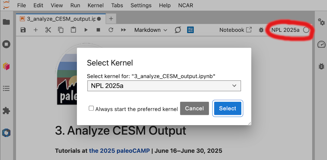
Figure: Select an NPL kernel
Load Python packages
import os
import glob
from datetime import timedelta

import xarray as xr
import numpy as np
import pandas as pd

import matplotlib as mpl
import matplotlib.pyplot as plt
import cartopy.crs as ccrs
from cartopy.util import add_cyclic_point

# geocat is used for interpolation of the atmosphere output
from geocat.comp import interpolation

# xesmf is used for regridding the ocean output
import xesmf

# hvplot provides interactive plots
import hvplot.xarray

import warnings
warnings.simplefilter("ignore", FutureWarning)
Analysis 1: plot solar insolation in the MH to further validate the simulation#
Load data#
I have both the piControl and midHolocene simulations finished.
I see 12-month history files for each simulation in my
Archive Directory.
!ls /glade/derecho/scratch/jiangzhu/archive/b.e21.B1850.f19_g17.piControl.001/atm/hist/*cam.h0.0001*
!ls /glade/derecho/scratch/jiangzhu/archive/b.e21.B1850.f19_g17.midHolocene.001/atm/hist/*cam.h0.0001*
/glade/derecho/scratch/jiangzhu/archive/b.e21.B1850.f19_g17.piControl.001/atm/hist/b.e21.B1850.f19_g17.piControl.001.cam.h0.0001-01.nc
/glade/derecho/scratch/jiangzhu/archive/b.e21.B1850.f19_g17.piControl.001/atm/hist/b.e21.B1850.f19_g17.piControl.001.cam.h0.0001-02.nc
/glade/derecho/scratch/jiangzhu/archive/b.e21.B1850.f19_g17.piControl.001/atm/hist/b.e21.B1850.f19_g17.piControl.001.cam.h0.0001-03.nc
/glade/derecho/scratch/jiangzhu/archive/b.e21.B1850.f19_g17.piControl.001/atm/hist/b.e21.B1850.f19_g17.piControl.001.cam.h0.0001-04.nc
/glade/derecho/scratch/jiangzhu/archive/b.e21.B1850.f19_g17.piControl.001/atm/hist/b.e21.B1850.f19_g17.piControl.001.cam.h0.0001-05.nc
/glade/derecho/scratch/jiangzhu/archive/b.e21.B1850.f19_g17.piControl.001/atm/hist/b.e21.B1850.f19_g17.piControl.001.cam.h0.0001-06.nc
/glade/derecho/scratch/jiangzhu/archive/b.e21.B1850.f19_g17.piControl.001/atm/hist/b.e21.B1850.f19_g17.piControl.001.cam.h0.0001-07.nc
/glade/derecho/scratch/jiangzhu/archive/b.e21.B1850.f19_g17.piControl.001/atm/hist/b.e21.B1850.f19_g17.piControl.001.cam.h0.0001-08.nc
/glade/derecho/scratch/jiangzhu/archive/b.e21.B1850.f19_g17.piControl.001/atm/hist/b.e21.B1850.f19_g17.piControl.001.cam.h0.0001-09.nc
/glade/derecho/scratch/jiangzhu/archive/b.e21.B1850.f19_g17.piControl.001/atm/hist/b.e21.B1850.f19_g17.piControl.001.cam.h0.0001-10.nc
/glade/derecho/scratch/jiangzhu/archive/b.e21.B1850.f19_g17.piControl.001/atm/hist/b.e21.B1850.f19_g17.piControl.001.cam.h0.0001-11.nc
/glade/derecho/scratch/jiangzhu/archive/b.e21.B1850.f19_g17.piControl.001/atm/hist/b.e21.B1850.f19_g17.piControl.001.cam.h0.0001-12.nc
/glade/derecho/scratch/jiangzhu/archive/b.e21.B1850.f19_g17.midHolocene.001/atm/hist/b.e21.B1850.f19_g17.midHolocene.001.cam.h0.0001-01.nc
/glade/derecho/scratch/jiangzhu/archive/b.e21.B1850.f19_g17.midHolocene.001/atm/hist/b.e21.B1850.f19_g17.midHolocene.001.cam.h0.0001-02.nc
/glade/derecho/scratch/jiangzhu/archive/b.e21.B1850.f19_g17.midHolocene.001/atm/hist/b.e21.B1850.f19_g17.midHolocene.001.cam.h0.0001-03.nc
/glade/derecho/scratch/jiangzhu/archive/b.e21.B1850.f19_g17.midHolocene.001/atm/hist/b.e21.B1850.f19_g17.midHolocene.001.cam.h0.0001-04.nc
/glade/derecho/scratch/jiangzhu/archive/b.e21.B1850.f19_g17.midHolocene.001/atm/hist/b.e21.B1850.f19_g17.midHolocene.001.cam.h0.0001-05.nc
/glade/derecho/scratch/jiangzhu/archive/b.e21.B1850.f19_g17.midHolocene.001/atm/hist/b.e21.B1850.f19_g17.midHolocene.001.cam.h0.0001-06.nc
/glade/derecho/scratch/jiangzhu/archive/b.e21.B1850.f19_g17.midHolocene.001/atm/hist/b.e21.B1850.f19_g17.midHolocene.001.cam.h0.0001-07.nc
/glade/derecho/scratch/jiangzhu/archive/b.e21.B1850.f19_g17.midHolocene.001/atm/hist/b.e21.B1850.f19_g17.midHolocene.001.cam.h0.0001-08.nc
/glade/derecho/scratch/jiangzhu/archive/b.e21.B1850.f19_g17.midHolocene.001/atm/hist/b.e21.B1850.f19_g17.midHolocene.001.cam.h0.0001-09.nc
/glade/derecho/scratch/jiangzhu/archive/b.e21.B1850.f19_g17.midHolocene.001/atm/hist/b.e21.B1850.f19_g17.midHolocene.001.cam.h0.0001-10.nc
/glade/derecho/scratch/jiangzhu/archive/b.e21.B1850.f19_g17.midHolocene.001/atm/hist/b.e21.B1850.f19_g17.midHolocene.001.cam.h0.0001-11.nc
/glade/derecho/scratch/jiangzhu/archive/b.e21.B1850.f19_g17.midHolocene.001/atm/hist/b.e21.B1850.f19_g17.midHolocene.001.cam.h0.0001-12.nc
Use
globandos.path.jointo obtain the file names including path.Use wildcard
*to catch all files in the atmosphere history directory (see Wildcard in 0.1_demo_unix.ipynb).
storage_dir = '/glade/derecho/scratch/jiangzhu/archive/'
hist_dir = 'atm/hist'

case_PI = 'b.e21.B1850.f19_g17.piControl.001'
case_MH = 'b.e21.B1850.f19_g17.midHolocene.001'

files_PI = glob.glob(os.path.join(storage_dir, case_PI, hist_dir, '*.cam.h0.0001*'))
files_MH = glob.glob(os.path.join(storage_dir, case_MH, hist_dir, '*.cam.h0.0001*'))

print('List of files for PI')
print(*files_PI, sep='\n')

print('List of files for MH')
print(*files_MH, sep='\n')
List of files for PI
/glade/derecho/scratch/jiangzhu/archive/b.e21.B1850.f19_g17.piControl.001/atm/hist/b.e21.B1850.f19_g17.piControl.001.cam.h0.0001-10.nc
/glade/derecho/scratch/jiangzhu/archive/b.e21.B1850.f19_g17.piControl.001/atm/hist/b.e21.B1850.f19_g17.piControl.001.cam.h0.0001-02.nc
/glade/derecho/scratch/jiangzhu/archive/b.e21.B1850.f19_g17.piControl.001/atm/hist/b.e21.B1850.f19_g17.piControl.001.cam.h0.0001-01.nc
/glade/derecho/scratch/jiangzhu/archive/b.e21.B1850.f19_g17.piControl.001/atm/hist/b.e21.B1850.f19_g17.piControl.001.cam.h0.0001-11.nc
/glade/derecho/scratch/jiangzhu/archive/b.e21.B1850.f19_g17.piControl.001/atm/hist/b.e21.B1850.f19_g17.piControl.001.cam.h0.0001-06.nc
/glade/derecho/scratch/jiangzhu/archive/b.e21.B1850.f19_g17.piControl.001/atm/hist/b.e21.B1850.f19_g17.piControl.001.cam.h0.0001-03.nc
/glade/derecho/scratch/jiangzhu/archive/b.e21.B1850.f19_g17.piControl.001/atm/hist/b.e21.B1850.f19_g17.piControl.001.cam.h0.0001-05.nc
/glade/derecho/scratch/jiangzhu/archive/b.e21.B1850.f19_g17.piControl.001/atm/hist/b.e21.B1850.f19_g17.piControl.001.cam.h0.0001-12.nc
/glade/derecho/scratch/jiangzhu/archive/b.e21.B1850.f19_g17.piControl.001/atm/hist/b.e21.B1850.f19_g17.piControl.001.cam.h0.0001-04.nc
/glade/derecho/scratch/jiangzhu/archive/b.e21.B1850.f19_g17.piControl.001/atm/hist/b.e21.B1850.f19_g17.piControl.001.cam.h0.0001-09.nc
/glade/derecho/scratch/jiangzhu/archive/b.e21.B1850.f19_g17.piControl.001/atm/hist/b.e21.B1850.f19_g17.piControl.001.cam.h0.0001-07.nc
/glade/derecho/scratch/jiangzhu/archive/b.e21.B1850.f19_g17.piControl.001/atm/hist/b.e21.B1850.f19_g17.piControl.001.cam.h0.0001-08.nc
List of files for MH
/glade/derecho/scratch/jiangzhu/archive/b.e21.B1850.f19_g17.midHolocene.001/atm/hist/b.e21.B1850.f19_g17.midHolocene.001.cam.h0.0001-04.nc
/glade/derecho/scratch/jiangzhu/archive/b.e21.B1850.f19_g17.midHolocene.001/atm/hist/b.e21.B1850.f19_g17.midHolocene.001.cam.h0.0001-06.nc
/glade/derecho/scratch/jiangzhu/archive/b.e21.B1850.f19_g17.midHolocene.001/atm/hist/b.e21.B1850.f19_g17.midHolocene.001.cam.h0.0001-07.nc
/glade/derecho/scratch/jiangzhu/archive/b.e21.B1850.f19_g17.midHolocene.001/atm/hist/b.e21.B1850.f19_g17.midHolocene.001.cam.h0.0001-03.nc
/glade/derecho/scratch/jiangzhu/archive/b.e21.B1850.f19_g17.midHolocene.001/atm/hist/b.e21.B1850.f19_g17.midHolocene.001.cam.h0.0001-11.nc
/glade/derecho/scratch/jiangzhu/archive/b.e21.B1850.f19_g17.midHolocene.001/atm/hist/b.e21.B1850.f19_g17.midHolocene.001.cam.h0.0001-08.nc
/glade/derecho/scratch/jiangzhu/archive/b.e21.B1850.f19_g17.midHolocene.001/atm/hist/b.e21.B1850.f19_g17.midHolocene.001.cam.h0.0001-01.nc
/glade/derecho/scratch/jiangzhu/archive/b.e21.B1850.f19_g17.midHolocene.001/atm/hist/b.e21.B1850.f19_g17.midHolocene.001.cam.h0.0001-05.nc
/glade/derecho/scratch/jiangzhu/archive/b.e21.B1850.f19_g17.midHolocene.001/atm/hist/b.e21.B1850.f19_g17.midHolocene.001.cam.h0.0001-02.nc
/glade/derecho/scratch/jiangzhu/archive/b.e21.B1850.f19_g17.midHolocene.001/atm/hist/b.e21.B1850.f19_g17.midHolocene.001.cam.h0.0001-09.nc
/glade/derecho/scratch/jiangzhu/archive/b.e21.B1850.f19_g17.midHolocene.001/atm/hist/b.e21.B1850.f19_g17.midHolocene.001.cam.h0.0001-12.nc
/glade/derecho/scratch/jiangzhu/archive/b.e21.B1850.f19_g17.midHolocene.001/atm/hist/b.e21.B1850.f19_g17.midHolocene.001.cam.h0.0001-10.nc
Use
xr.open_mfdatasetto open multiple files at once in parallel (12 months in this case)We will keep using the Xarray Datasets
ds_MHandds_PIthroughout the Notebook
ds_PI = xr.open_mfdataset(
    files_PI,
    combine="by_coords",
    data_vars="minimal",
    coords="minimal",
    compat="override",
)

ds_MH = xr.open_mfdataset(
    files_MH,
    combine="by_coords",
    data_vars="minimal",
    coords="minimal",
    compat="override",
)

ds_PI
<xarray.Dataset> Size: 541MB
Dimensions:       (zlon: 1, nbnd: 2, lat: 96, lev: 26, ilev: 27, time: 12,
                   lon: 144)
Coordinates:
  * zlon          (zlon) float64 8B 0.0
  * lat           (lat) float64 768B -90.0 -88.11 -86.21 ... 86.21 88.11 90.0
  * lev           (lev) float64 208B 3.545 7.389 13.97 ... 929.6 970.6 992.6
  * ilev          (ilev) float64 216B 2.194 4.895 9.882 ... 956.0 985.1 1e+03
  * time          (time) object 96B 0001-02-01 00:00:00 ... 0002-01-01 00:00:00
  * lon           (lon) float64 1kB 0.0 2.5 5.0 7.5 ... 350.0 352.5 355.0 357.5
Dimensions without coordinates: nbnd
Data variables: (12/122)
    zlon_bnds     (zlon, nbnd) float64 16B dask.array<chunksize=(1, 2), meta=np.ndarray>
    gw            (lat) float64 768B dask.array<chunksize=(96,), meta=np.ndarray>
    hyam          (lev) float64 208B dask.array<chunksize=(26,), meta=np.ndarray>
    hybm          (lev) float64 208B dask.array<chunksize=(26,), meta=np.ndarray>
    P0            float64 8B ...
    hyai          (ilev) float64 216B dask.array<chunksize=(27,), meta=np.ndarray>
    ...            ...
    VU            (time, lev, lat, lon) float32 17MB dask.array<chunksize=(1, 26, 96, 144), meta=np.ndarray>
    VV            (time, lev, lat, lon) float32 17MB dask.array<chunksize=(1, 26, 96, 144), meta=np.ndarray>
    Vzm           (time, ilev, lat, zlon) float32 124kB dask.array<chunksize=(1, 27, 96, 1), meta=np.ndarray>
    WTHzm         (time, ilev, lat, zlon) float32 124kB dask.array<chunksize=(1, 27, 96, 1), meta=np.ndarray>
    Wzm           (time, ilev, lat, zlon) float32 124kB dask.array<chunksize=(1, 27, 96, 1), meta=np.ndarray>
    Z3            (time, lev, lat, lon) float32 17MB dask.array<chunksize=(1, 26, 96, 144), meta=np.ndarray>
Attributes:
    Conventions:       CF-1.0
    source:            CAM
    case:              b.e21.B1850.f19_g17.piControl.001
    logname:           jiangzhu
    host:              derecho3
    initial_file:      /glade/campaign/cesm/cesmdata/inputdata/atm/cam/inic/f...
    topography_file:   /glade/campaign/cesm/cesmdata/inputdata/atm/cam/topo/f...
    model_doi_url:     https://doi.org/10.5065/D67H1H0V
time_period_freq: month_1- zlon: 1
- nbnd: 2
- lat: 96
- lev: 26
- ilev: 27
- time: 12
- lon: 144
- zlon(zlon)float640.0
- long_name :
- longitude
- units :
- degrees_east
- bounds :
- zlon_bnds
array([0.])
- lat(lat)float64-90.0 -88.11 -86.21 ... 88.11 90.0
- long_name :
- latitude
- units :
- degrees_north
array([-90. , -88.105263, -86.210526, -84.315789, -82.421053, -80.526316, -78.631579, -76.736842, -74.842105, -72.947368, -71.052632, -69.157895, -67.263158, -65.368421, -63.473684, -61.578947, -59.684211, -57.789474, -55.894737, -54. , -52.105263, -50.210526, -48.315789, -46.421053, -44.526316, -42.631579, -40.736842, -38.842105, -36.947368, -35.052632, -33.157895, -31.263158, -29.368421, -27.473684, -25.578947, -23.684211, -21.789474, -19.894737, -18. , -16.105263, -14.210526, -12.315789, -10.421053, -8.526316, -6.631579, -4.736842, -2.842105, -0.947368, 0.947368, 2.842105, 4.736842, 6.631579, 8.526316, 10.421053, 12.315789, 14.210526, 16.105263, 18. , 19.894737, 21.789474, 23.684211, 25.578947, 27.473684, 29.368421, 31.263158, 33.157895, 35.052632, 36.947368, 38.842105, 40.736842, 42.631579, 44.526316, 46.421053, 48.315789, 50.210526, 52.105263, 54. , 55.894737, 57.789474, 59.684211, 61.578947, 63.473684, 65.368421, 67.263158, 69.157895, 71.052632, 72.947368, 74.842105, 76.736842, 78.631579, 80.526316, 82.421053, 84.315789, 86.210526, 88.105263, 90. ]) - lev(lev)float643.545 7.389 13.97 ... 970.6 992.6
- long_name :
- hybrid level at midpoints (1000*(A+B))
- units :
- hPa
- positive :
- down
- standard_name :
- atmosphere_hybrid_sigma_pressure_coordinate
- formula_terms :
- a: hyam b: hybm p0: P0 ps: PS
array([ 3.544638, 7.388814, 13.967214, 23.944625, 37.23029 , 53.114605, 70.05915 , 85.439115, 100.514695, 118.250335, 139.115395, 163.66207 , 192.539935, 226.513265, 266.481155, 313.501265, 368.81798 , 433.895225, 510.455255, 600.5242 , 696.79629 , 787.70206 , 867.16076 , 929.648875, 970.55483 , 992.5561 ]) - ilev(ilev)float642.194 4.895 9.882 ... 985.1 1e+03
- long_name :
- hybrid level at interfaces (1000*(A+B))
- units :
- hPa
- positive :
- down
- standard_name :
- atmosphere_hybrid_sigma_pressure_coordinate
- formula_terms :
- a: hyai b: hybi p0: P0 ps: PS
array([ 2.194067, 4.895209, 9.882418, 18.05201 , 29.83724 , 44.62334 , 61.60587 , 78.51243 , 92.3658 , 108.66359 , 127.83708 , 150.39371 , 176.93043 , 208.14944 , 244.87709 , 288.08522 , 338.91731 , 398.71865 , 469.0718 , 551.83871 , 649.20969 , 744.38289 , 831.02123 , 903.30029 , 955.99746 , 985.1122 , 1000. ]) - time(time)object0001-02-01 00:00:00 ... 0002-01-...
- long_name :
- time
- bounds :
- time_bnds
array([cftime.DatetimeNoLeap(1, 2, 1, 0, 0, 0, 0, has_year_zero=True), cftime.DatetimeNoLeap(1, 3, 1, 0, 0, 0, 0, has_year_zero=True), cftime.DatetimeNoLeap(1, 4, 1, 0, 0, 0, 0, has_year_zero=True), cftime.DatetimeNoLeap(1, 5, 1, 0, 0, 0, 0, has_year_zero=True), cftime.DatetimeNoLeap(1, 6, 1, 0, 0, 0, 0, has_year_zero=True), cftime.DatetimeNoLeap(1, 7, 1, 0, 0, 0, 0, has_year_zero=True), cftime.DatetimeNoLeap(1, 8, 1, 0, 0, 0, 0, has_year_zero=True), cftime.DatetimeNoLeap(1, 9, 1, 0, 0, 0, 0, has_year_zero=True), cftime.DatetimeNoLeap(1, 10, 1, 0, 0, 0, 0, has_year_zero=True), cftime.DatetimeNoLeap(1, 11, 1, 0, 0, 0, 0, has_year_zero=True), cftime.DatetimeNoLeap(1, 12, 1, 0, 0, 0, 0, has_year_zero=True), cftime.DatetimeNoLeap(2, 1, 1, 0, 0, 0, 0, has_year_zero=True)], dtype=object) - lon(lon)float640.0 2.5 5.0 ... 352.5 355.0 357.5
- long_name :
- longitude
- units :
- degrees_east
array([  0. ,   2.5,   5. ,   7.5,  10. ,  12.5,  15. ,  17.5,  20. ,  22.5,
        25. ,  27.5,  30. ,  32.5,  35. ,  37.5,  40. ,  42.5,  45. ,  47.5,
        50. ,  52.5,  55. ,  57.5,  60. ,  62.5,  65. ,  67.5,  70. ,  72.5,
        75. ,  77.5,  80. ,  82.5,  85. ,  87.5,  90. ,  92.5,  95. ,  97.5,
       100. , 102.5, 105. , 107.5, 110. , 112.5, 115. , 117.5, 120. , 122.5,
       125. , 127.5, 130. , 132.5, 135. , 137.5, 140. , 142.5, 145. , 147.5,
       150. , 152.5, 155. , 157.5, 160. , 162.5, 165. , 167.5, 170. , 172.5,
       175. , 177.5, 180. , 182.5, 185. , 187.5, 190. , 192.5, 195. , 197.5,
       200. , 202.5, 205. , 207.5, 210. , 212.5, 215. , 217.5, 220. , 222.5,
       225. , 227.5, 230. , 232.5, 235. , 237.5, 240. , 242.5, 245. , 247.5,
       250. , 252.5, 255. , 257.5, 260. , 262.5, 265. , 267.5, 270. , 272.5,
       275. , 277.5, 280. , 282.5, 285. , 287.5, 290. , 292.5, 295. , 297.5,
       300. , 302.5, 305. , 307.5, 310. , 312.5, 315. , 317.5, 320. , 322.5,
       325. , 327.5, 330. , 332.5, 335. , 337.5, 340. , 342.5, 345. , 347.5,
       350. , 352.5, 355. , 357.5])
- zlon_bnds(zlon, nbnd)float64dask.array<chunksize=(1, 2), meta=np.ndarray>
- long_name :
- zlon bounds
- units :
- degrees_east
Array Chunk Bytes 16 B 16 B Shape (1, 2) (1, 2) Dask graph 1 chunks in 2 graph layers Data type float64 numpy.ndarray - gw(lat)float64dask.array<chunksize=(96,), meta=np.ndarray>
- long_name :
- latitude weights
Array Chunk Bytes 768 B 768 B Shape (96,) (96,) Dask graph 1 chunks in 2 graph layers Data type float64 numpy.ndarray - hyam(lev)float64dask.array<chunksize=(26,), meta=np.ndarray>
- long_name :
- hybrid A coefficient at layer midpoints
Array Chunk Bytes 208 B 208 B Shape (26,) (26,) Dask graph 1 chunks in 2 graph layers Data type float64 numpy.ndarray - hybm(lev)float64dask.array<chunksize=(26,), meta=np.ndarray>
- long_name :
- hybrid B coefficient at layer midpoints
Array Chunk Bytes 208 B 208 B Shape (26,) (26,) Dask graph 1 chunks in 2 graph layers Data type float64 numpy.ndarray - P0()float64...
- long_name :
- reference pressure
- units :
- Pa
[1 values with dtype=float64]
- hyai(ilev)float64dask.array<chunksize=(27,), meta=np.ndarray>
- long_name :
- hybrid A coefficient at layer interfaces
Array Chunk Bytes 216 B 216 B Shape (27,) (27,) Dask graph 1 chunks in 2 graph layers Data type float64 numpy.ndarray - hybi(ilev)float64dask.array<chunksize=(27,), meta=np.ndarray>
- long_name :
- hybrid B coefficient at layer interfaces
Array Chunk Bytes 216 B 216 B Shape (27,) (27,) Dask graph 1 chunks in 2 graph layers Data type float64 numpy.ndarray - date(time)int32dask.array<chunksize=(1,), meta=np.ndarray>
- long_name :
- current date (YYYYMMDD)
Array Chunk Bytes 48 B 4 B Shape (12,) (1,) Dask graph 12 chunks in 25 graph layers Data type int32 numpy.ndarray - datesec(time)int32dask.array<chunksize=(1,), meta=np.ndarray>
- long_name :
- current seconds of current date
Array Chunk Bytes 48 B 4 B Shape (12,) (1,) Dask graph 12 chunks in 25 graph layers Data type int32 numpy.ndarray - time_bnds(time, nbnd)objectdask.array<chunksize=(1, 2), meta=np.ndarray>
- long_name :
- time interval endpoints
Array Chunk Bytes 192 B 16 B Shape (12, 2) (1, 2) Dask graph 12 chunks in 25 graph layers Data type object numpy.ndarray - date_written(time)|S8dask.array<chunksize=(1,), meta=np.ndarray>
Array Chunk Bytes 96 B 8 B Shape (12,) (1,) Dask graph 12 chunks in 37 graph layers Data type |S8 numpy.ndarray - time_written(time)|S8dask.array<chunksize=(1,), meta=np.ndarray>
Array Chunk Bytes 96 B 8 B Shape (12,) (1,) Dask graph 12 chunks in 37 graph layers Data type |S8 numpy.ndarray - ndbase()int32...
- long_name :
- base day
[1 values with dtype=int32]
- nsbase()int32...
- long_name :
- seconds of base day
[1 values with dtype=int32]
- nbdate()int32...
- long_name :
- base date (YYYYMMDD)
[1 values with dtype=int32]
- nbsec()int32...
- long_name :
- seconds of base date
[1 values with dtype=int32]
- mdt()int32...
- long_name :
- timestep
- units :
- s
[1 values with dtype=int32]
- ndcur(time)int32dask.array<chunksize=(1,), meta=np.ndarray>
- long_name :
- current day (from base day)
Array Chunk Bytes 48 B 4 B Shape (12,) (1,) Dask graph 12 chunks in 25 graph layers Data type int32 numpy.ndarray - nscur(time)int32dask.array<chunksize=(1,), meta=np.ndarray>
- long_name :
- current seconds of current day
Array Chunk Bytes 48 B 4 B Shape (12,) (1,) Dask graph 12 chunks in 25 graph layers Data type int32 numpy.ndarray - co2vmr(time)float64dask.array<chunksize=(1,), meta=np.ndarray>
- long_name :
- co2 volume mixing ratio
Array Chunk Bytes 96 B 8 B Shape (12,) (1,) Dask graph 12 chunks in 25 graph layers Data type float64 numpy.ndarray - ch4vmr(time)float64dask.array<chunksize=(1,), meta=np.ndarray>
- long_name :
- ch4 volume mixing ratio
Array Chunk Bytes 96 B 8 B Shape (12,) (1,) Dask graph 12 chunks in 25 graph layers Data type float64 numpy.ndarray - n2ovmr(time)float64dask.array<chunksize=(1,), meta=np.ndarray>
- long_name :
- n2o volume mixing ratio
Array Chunk Bytes 96 B 8 B Shape (12,) (1,) Dask graph 12 chunks in 25 graph layers Data type float64 numpy.ndarray - f11vmr(time)float64dask.array<chunksize=(1,), meta=np.ndarray>
- long_name :
- f11 volume mixing ratio
Array Chunk Bytes 96 B 8 B Shape (12,) (1,) Dask graph 12 chunks in 25 graph layers Data type float64 numpy.ndarray - f12vmr(time)float64dask.array<chunksize=(1,), meta=np.ndarray>
- long_name :
- f12 volume mixing ratio
Array Chunk Bytes 96 B 8 B Shape (12,) (1,) Dask graph 12 chunks in 25 graph layers Data type float64 numpy.ndarray - sol_tsi(time)float64dask.array<chunksize=(1,), meta=np.ndarray>
- long_name :
- total solar irradiance
- units :
- W/m2
Array Chunk Bytes 96 B 8 B Shape (12,) (1,) Dask graph 12 chunks in 25 graph layers Data type float64 numpy.ndarray - nsteph(time)int32dask.array<chunksize=(1,), meta=np.ndarray>
- long_name :
- current timestep
Array Chunk Bytes 48 B 4 B Shape (12,) (1,) Dask graph 12 chunks in 25 graph layers Data type int32 numpy.ndarray - AEROD_v(time, lat, lon)float32dask.array<chunksize=(1, 96, 144), meta=np.ndarray>
- units :
- 1
- long_name :
- Total Aerosol Optical Depth in visible band
- cell_methods :
- time: mean
Array Chunk Bytes 648.00 kiB 54.00 kiB Shape (12, 96, 144) (1, 96, 144) Dask graph 12 chunks in 25 graph layers Data type float32 numpy.ndarray - CLDHGH(time, lat, lon)float32dask.array<chunksize=(1, 96, 144), meta=np.ndarray>
- Sampling_Sequence :
- rad_lwsw
- units :
- fraction
- long_name :
- Vertically-integrated high cloud
- cell_methods :
- time: mean
Array Chunk Bytes 648.00 kiB 54.00 kiB Shape (12, 96, 144) (1, 96, 144) Dask graph 12 chunks in 25 graph layers Data type float32 numpy.ndarray - CLDICE(time, lev, lat, lon)float32dask.array<chunksize=(1, 26, 96, 144), meta=np.ndarray>
- mdims :
- 1
- units :
- kg/kg
- mixing_ratio :
- wet
- long_name :
- Grid box averaged cloud ice amount
- cell_methods :
- time: mean
Array Chunk Bytes 16.45 MiB 1.37 MiB Shape (12, 26, 96, 144) (1, 26, 96, 144) Dask graph 12 chunks in 25 graph layers Data type float32 numpy.ndarray - CLDLIQ(time, lev, lat, lon)float32dask.array<chunksize=(1, 26, 96, 144), meta=np.ndarray>
- mdims :
- 1
- units :
- kg/kg
- mixing_ratio :
- wet
- long_name :
- Grid box averaged cloud liquid amount
- cell_methods :
- time: mean
Array Chunk Bytes 16.45 MiB 1.37 MiB Shape (12, 26, 96, 144) (1, 26, 96, 144) Dask graph 12 chunks in 25 graph layers Data type float32 numpy.ndarray - CLDLOW(time, lat, lon)float32dask.array<chunksize=(1, 96, 144), meta=np.ndarray>
- Sampling_Sequence :
- rad_lwsw
- units :
- fraction
- long_name :
- Vertically-integrated low cloud
- cell_methods :
- time: mean
Array Chunk Bytes 648.00 kiB 54.00 kiB Shape (12, 96, 144) (1, 96, 144) Dask graph 12 chunks in 25 graph layers Data type float32 numpy.ndarray - CLDMED(time, lat, lon)float32dask.array<chunksize=(1, 96, 144), meta=np.ndarray>
- Sampling_Sequence :
- rad_lwsw
- units :
- fraction
- long_name :
- Vertically-integrated mid-level cloud
- cell_methods :
- time: mean
Array Chunk Bytes 648.00 kiB 54.00 kiB Shape (12, 96, 144) (1, 96, 144) Dask graph 12 chunks in 25 graph layers Data type float32 numpy.ndarray - CLDTOT(time, lat, lon)float32dask.array<chunksize=(1, 96, 144), meta=np.ndarray>
- Sampling_Sequence :
- rad_lwsw
- units :
- fraction
- long_name :
- Vertically-integrated total cloud
- cell_methods :
- time: mean
Array Chunk Bytes 648.00 kiB 54.00 kiB Shape (12, 96, 144) (1, 96, 144) Dask graph 12 chunks in 25 graph layers Data type float32 numpy.ndarray - CLOUD(time, lev, lat, lon)float32dask.array<chunksize=(1, 26, 96, 144), meta=np.ndarray>
- mdims :
- 1
- Sampling_Sequence :
- rad_lwsw
- units :
- fraction
- long_name :
- Cloud fraction
- cell_methods :
- time: mean
Array Chunk Bytes 16.45 MiB 1.37 MiB Shape (12, 26, 96, 144) (1, 26, 96, 144) Dask graph 12 chunks in 25 graph layers Data type float32 numpy.ndarray - CONCLD(time, lev, lat, lon)float32dask.array<chunksize=(1, 26, 96, 144), meta=np.ndarray>
- mdims :
- 1
- units :
- fraction
- long_name :
- Convective cloud cover
- cell_methods :
- time: mean
Array Chunk Bytes 16.45 MiB 1.37 MiB Shape (12, 26, 96, 144) (1, 26, 96, 144) Dask graph 12 chunks in 25 graph layers Data type float32 numpy.ndarray - DCQ(time, lev, lat, lon)float32dask.array<chunksize=(1, 26, 96, 144), meta=np.ndarray>
- mdims :
- 1
- units :
- kg/kg/s
- long_name :
- Q tendency due to moist processes
- cell_methods :
- time: mean
Array Chunk Bytes 16.45 MiB 1.37 MiB Shape (12, 26, 96, 144) (1, 26, 96, 144) Dask graph 12 chunks in 25 graph layers Data type float32 numpy.ndarray - DTCOND(time, lev, lat, lon)float32dask.array<chunksize=(1, 26, 96, 144), meta=np.ndarray>
- mdims :
- 1
- units :
- K/s
- long_name :
- T tendency - moist processes
- cell_methods :
- time: mean
Array Chunk Bytes 16.45 MiB 1.37 MiB Shape (12, 26, 96, 144) (1, 26, 96, 144) Dask graph 12 chunks in 25 graph layers Data type float32 numpy.ndarray - DTV(time, lev, lat, lon)float32dask.array<chunksize=(1, 26, 96, 144), meta=np.ndarray>
- mdims :
- 1
- units :
- K/s
- long_name :
- T vertical diffusion
- cell_methods :
- time: mean
Array Chunk Bytes 16.45 MiB 1.37 MiB Shape (12, 26, 96, 144) (1, 26, 96, 144) Dask graph 12 chunks in 25 graph layers Data type float32 numpy.ndarray - EMIS(time, lev, lat, lon)float32dask.array<chunksize=(1, 26, 96, 144), meta=np.ndarray>
- mdims :
- 1
- Sampling_Sequence :
- rad_lwsw
- units :
- 1
- long_name :
- cloud emissivity
- cell_methods :
- time: mean
Array Chunk Bytes 16.45 MiB 1.37 MiB Shape (12, 26, 96, 144) (1, 26, 96, 144) Dask graph 12 chunks in 25 graph layers Data type float32 numpy.ndarray - FICE(time, lev, lat, lon)float32dask.array<chunksize=(1, 26, 96, 144), meta=np.ndarray>
- mdims :
- 1
- units :
- fraction
- long_name :
- Fractional ice content within cloud
- cell_methods :
- time: mean
Array Chunk Bytes 16.45 MiB 1.37 MiB Shape (12, 26, 96, 144) (1, 26, 96, 144) Dask graph 12 chunks in 25 graph layers Data type float32 numpy.ndarray - FLDS(time, lat, lon)float32dask.array<chunksize=(1, 96, 144), meta=np.ndarray>
- Sampling_Sequence :
- rad_lwsw
- units :
- W/m2
- long_name :
- Downwelling longwave flux at surface
- cell_methods :
- time: mean
Array Chunk Bytes 648.00 kiB 54.00 kiB Shape (12, 96, 144) (1, 96, 144) Dask graph 12 chunks in 25 graph layers Data type float32 numpy.ndarray - FLDSC(time, lat, lon)float32dask.array<chunksize=(1, 96, 144), meta=np.ndarray>
- Sampling_Sequence :
- rad_lwsw
- units :
- W/m2
- long_name :
- Clearsky downwelling longwave flux at surface
- cell_methods :
- time: mean
Array Chunk Bytes 648.00 kiB 54.00 kiB Shape (12, 96, 144) (1, 96, 144) Dask graph 12 chunks in 25 graph layers Data type float32 numpy.ndarray - FLNS(time, lat, lon)float32dask.array<chunksize=(1, 96, 144), meta=np.ndarray>
- Sampling_Sequence :
- rad_lwsw
- units :
- W/m2
- long_name :
- Net longwave flux at surface
- cell_methods :
- time: mean
Array Chunk Bytes 648.00 kiB 54.00 kiB Shape (12, 96, 144) (1, 96, 144) Dask graph 12 chunks in 25 graph layers Data type float32 numpy.ndarray - FLNSC(time, lat, lon)float32dask.array<chunksize=(1, 96, 144), meta=np.ndarray>
- Sampling_Sequence :
- rad_lwsw
- units :
- W/m2
- long_name :
- Clearsky net longwave flux at surface
- cell_methods :
- time: mean
Array Chunk Bytes 648.00 kiB 54.00 kiB Shape (12, 96, 144) (1, 96, 144) Dask graph 12 chunks in 25 graph layers Data type float32 numpy.ndarray - FLNT(time, lat, lon)float32dask.array<chunksize=(1, 96, 144), meta=np.ndarray>
- Sampling_Sequence :
- rad_lwsw
- units :
- W/m2
- long_name :
- Net longwave flux at top of model
- cell_methods :
- time: mean
Array Chunk Bytes 648.00 kiB 54.00 kiB Shape (12, 96, 144) (1, 96, 144) Dask graph 12 chunks in 25 graph layers Data type float32 numpy.ndarray - FLNTC(time, lat, lon)float32dask.array<chunksize=(1, 96, 144), meta=np.ndarray>
- Sampling_Sequence :
- rad_lwsw
- units :
- W/m2
- long_name :
- Clearsky net longwave flux at top of model
- cell_methods :
- time: mean
Array Chunk Bytes 648.00 kiB 54.00 kiB Shape (12, 96, 144) (1, 96, 144) Dask graph 12 chunks in 25 graph layers Data type float32 numpy.ndarray - FLUT(time, lat, lon)float32dask.array<chunksize=(1, 96, 144), meta=np.ndarray>
- Sampling_Sequence :
- rad_lwsw
- units :
- W/m2
- long_name :
- Upwelling longwave flux at top of model
- cell_methods :
- time: mean
Array Chunk Bytes 648.00 kiB 54.00 kiB Shape (12, 96, 144) (1, 96, 144) Dask graph 12 chunks in 25 graph layers Data type float32 numpy.ndarray - FLUTC(time, lat, lon)float32dask.array<chunksize=(1, 96, 144), meta=np.ndarray>
- Sampling_Sequence :
- rad_lwsw
- units :
- W/m2
- long_name :
- Clearsky upwelling longwave flux at top of model
- cell_methods :
- time: mean
Array Chunk Bytes 648.00 kiB 54.00 kiB Shape (12, 96, 144) (1, 96, 144) Dask graph 12 chunks in 25 graph layers Data type float32 numpy.ndarray - FSDS(time, lat, lon)float32dask.array<chunksize=(1, 96, 144), meta=np.ndarray>
- Sampling_Sequence :
- rad_lwsw
- units :
- W/m2
- long_name :
- Downwelling solar flux at surface
- cell_methods :
- time: mean
Array Chunk Bytes 648.00 kiB 54.00 kiB Shape (12, 96, 144) (1, 96, 144) Dask graph 12 chunks in 25 graph layers Data type float32 numpy.ndarray - FSDSC(time, lat, lon)float32dask.array<chunksize=(1, 96, 144), meta=np.ndarray>
- Sampling_Sequence :
- rad_lwsw
- units :
- W/m2
- long_name :
- Clearsky downwelling solar flux at surface
- cell_methods :
- time: mean
Array Chunk Bytes 648.00 kiB 54.00 kiB Shape (12, 96, 144) (1, 96, 144) Dask graph 12 chunks in 25 graph layers Data type float32 numpy.ndarray - FSDTOA(time, lat, lon)float32dask.array<chunksize=(1, 96, 144), meta=np.ndarray>
- Sampling_Sequence :
- rad_lwsw
- units :
- W/m2
- long_name :
- Downwelling solar flux at top of atmosphere
- cell_methods :
- time: mean
Array Chunk Bytes 648.00 kiB 54.00 kiB Shape (12, 96, 144) (1, 96, 144) Dask graph 12 chunks in 25 graph layers Data type float32 numpy.ndarray - FSNS(time, lat, lon)float32dask.array<chunksize=(1, 96, 144), meta=np.ndarray>
- Sampling_Sequence :
- rad_lwsw
- units :
- W/m2
- long_name :
- Net solar flux at surface
- cell_methods :
- time: mean
Array Chunk Bytes 648.00 kiB 54.00 kiB Shape (12, 96, 144) (1, 96, 144) Dask graph 12 chunks in 25 graph layers Data type float32 numpy.ndarray - FSNSC(time, lat, lon)float32dask.array<chunksize=(1, 96, 144), meta=np.ndarray>
- Sampling_Sequence :
- rad_lwsw
- units :
- W/m2
- long_name :
- Clearsky net solar flux at surface
- cell_methods :
- time: mean
Array Chunk Bytes 648.00 kiB 54.00 kiB Shape (12, 96, 144) (1, 96, 144) Dask graph 12 chunks in 25 graph layers Data type float32 numpy.ndarray - FSNT(time, lat, lon)float32dask.array<chunksize=(1, 96, 144), meta=np.ndarray>
- Sampling_Sequence :
- rad_lwsw
- units :
- W/m2
- long_name :
- Net solar flux at top of model
- cell_methods :
- time: mean
Array Chunk Bytes 648.00 kiB 54.00 kiB Shape (12, 96, 144) (1, 96, 144) Dask graph 12 chunks in 25 graph layers Data type float32 numpy.ndarray - FSNTC(time, lat, lon)float32dask.array<chunksize=(1, 96, 144), meta=np.ndarray>
- Sampling_Sequence :
- rad_lwsw
- units :
- W/m2
- long_name :
- Clearsky net solar flux at top of model
- cell_methods :
- time: mean
Array Chunk Bytes 648.00 kiB 54.00 kiB Shape (12, 96, 144) (1, 96, 144) Dask graph 12 chunks in 25 graph layers Data type float32 numpy.ndarray - FSNTOA(time, lat, lon)float32dask.array<chunksize=(1, 96, 144), meta=np.ndarray>
- Sampling_Sequence :
- rad_lwsw
- units :
- W/m2
- long_name :
- Net solar flux at top of atmosphere
- cell_methods :
- time: mean
Array Chunk Bytes 648.00 kiB 54.00 kiB Shape (12, 96, 144) (1, 96, 144) Dask graph 12 chunks in 25 graph layers Data type float32 numpy.ndarray - FSNTOAC(time, lat, lon)float32dask.array<chunksize=(1, 96, 144), meta=np.ndarray>
- Sampling_Sequence :
- rad_lwsw
- units :
- W/m2
- long_name :
- Clearsky net solar flux at top of atmosphere
- cell_methods :
- time: mean
Array Chunk Bytes 648.00 kiB 54.00 kiB Shape (12, 96, 144) (1, 96, 144) Dask graph 12 chunks in 25 graph layers Data type float32 numpy.ndarray - FSUTOA(time, lat, lon)float32dask.array<chunksize=(1, 96, 144), meta=np.ndarray>
- Sampling_Sequence :
- rad_lwsw
- units :
- W/m2
- long_name :
- Upwelling solar flux at top of atmosphere
- cell_methods :
- time: mean
Array Chunk Bytes 648.00 kiB 54.00 kiB Shape (12, 96, 144) (1, 96, 144) Dask graph 12 chunks in 25 graph layers Data type float32 numpy.ndarray - ICEFRAC(time, lat, lon)float32dask.array<chunksize=(1, 96, 144), meta=np.ndarray>
- units :
- fraction
- long_name :
- Fraction of sfc area covered by sea-ice
- cell_methods :
- time: mean
Array Chunk Bytes 648.00 kiB 54.00 kiB Shape (12, 96, 144) (1, 96, 144) Dask graph 12 chunks in 25 graph layers Data type float32 numpy.ndarray - ICIMR(time, lev, lat, lon)float32dask.array<chunksize=(1, 26, 96, 144), meta=np.ndarray>
- mdims :
- 1
- units :
- kg/kg
- long_name :
- Prognostic in-cloud ice mixing ratio
- cell_methods :
- time: mean
Array Chunk Bytes 16.45 MiB 1.37 MiB Shape (12, 26, 96, 144) (1, 26, 96, 144) Dask graph 12 chunks in 25 graph layers Data type float32 numpy.ndarray - ICWMR(time, lev, lat, lon)float32dask.array<chunksize=(1, 26, 96, 144), meta=np.ndarray>
- mdims :
- 1
- units :
- kg/kg
- long_name :
- Prognostic in-cloud water mixing ratio
- cell_methods :
- time: mean
Array Chunk Bytes 16.45 MiB 1.37 MiB Shape (12, 26, 96, 144) (1, 26, 96, 144) Dask graph 12 chunks in 25 graph layers Data type float32 numpy.ndarray - LANDFRAC(time, lat, lon)float32dask.array<chunksize=(1, 96, 144), meta=np.ndarray>
- units :
- fraction
- long_name :
- Fraction of sfc area covered by land
- cell_methods :
- time: mean
Array Chunk Bytes 648.00 kiB 54.00 kiB Shape (12, 96, 144) (1, 96, 144) Dask graph 12 chunks in 25 graph layers Data type float32 numpy.ndarray - LHFLX(time, lat, lon)float32dask.array<chunksize=(1, 96, 144), meta=np.ndarray>
- units :
- W/m2
- long_name :
- Surface latent heat flux
- cell_methods :
- time: mean
Array Chunk Bytes 648.00 kiB 54.00 kiB Shape (12, 96, 144) (1, 96, 144) Dask graph 12 chunks in 25 graph layers Data type float32 numpy.ndarray - LWCF(time, lat, lon)float32dask.array<chunksize=(1, 96, 144), meta=np.ndarray>
- Sampling_Sequence :
- rad_lwsw
- units :
- W/m2
- long_name :
- Longwave cloud forcing
- cell_methods :
- time: mean
Array Chunk Bytes 648.00 kiB 54.00 kiB Shape (12, 96, 144) (1, 96, 144) Dask graph 12 chunks in 25 graph layers Data type float32 numpy.ndarray - MSKtem(time, lat, lon)float32dask.array<chunksize=(1, 96, 144), meta=np.ndarray>
- units :
- 1
- long_name :
- TEM mask
- cell_methods :
- time: mean
Array Chunk Bytes 648.00 kiB 54.00 kiB Shape (12, 96, 144) (1, 96, 144) Dask graph 12 chunks in 25 graph layers Data type float32 numpy.ndarray - OCNFRAC(time, lat, lon)float32dask.array<chunksize=(1, 96, 144), meta=np.ndarray>
- units :
- fraction
- long_name :
- Fraction of sfc area covered by ocean
- cell_methods :
- time: mean
Array Chunk Bytes 648.00 kiB 54.00 kiB Shape (12, 96, 144) (1, 96, 144) Dask graph 12 chunks in 25 graph layers Data type float32 numpy.ndarray - OMEGA(time, lev, lat, lon)float32dask.array<chunksize=(1, 26, 96, 144), meta=np.ndarray>
- mdims :
- 1
- units :
- Pa/s
- long_name :
- Vertical velocity (pressure)
- cell_methods :
- time: mean
Array Chunk Bytes 16.45 MiB 1.37 MiB Shape (12, 26, 96, 144) (1, 26, 96, 144) Dask graph 12 chunks in 25 graph layers Data type float32 numpy.ndarray - OMEGAT(time, lev, lat, lon)float32dask.array<chunksize=(1, 26, 96, 144), meta=np.ndarray>
- mdims :
- 1
- units :
- K Pa/s
- long_name :
- Vertical heat flux
- cell_methods :
- time: mean
Array Chunk Bytes 16.45 MiB 1.37 MiB Shape (12, 26, 96, 144) (1, 26, 96, 144) Dask graph 12 chunks in 25 graph layers Data type float32 numpy.ndarray - PBLH(time, lat, lon)float32dask.array<chunksize=(1, 96, 144), meta=np.ndarray>
- units :
- m
- long_name :
- PBL height
- cell_methods :
- time: mean
Array Chunk Bytes 648.00 kiB 54.00 kiB Shape (12, 96, 144) (1, 96, 144) Dask graph 12 chunks in 25 graph layers Data type float32 numpy.ndarray - PHIS(time, lat, lon)float32dask.array<chunksize=(1, 96, 144), meta=np.ndarray>
- units :
- m2/s2
- long_name :
- Surface geopotential
Array Chunk Bytes 648.00 kiB 54.00 kiB Shape (12, 96, 144) (1, 96, 144) Dask graph 12 chunks in 25 graph layers Data type float32 numpy.ndarray - PRECC(time, lat, lon)float32dask.array<chunksize=(1, 96, 144), meta=np.ndarray>
- units :
- m/s
- long_name :
- Convective precipitation rate (liq + ice)
- cell_methods :
- time: mean
Array Chunk Bytes 648.00 kiB 54.00 kiB Shape (12, 96, 144) (1, 96, 144) Dask graph 12 chunks in 25 graph layers Data type float32 numpy.ndarray - PRECL(time, lat, lon)float32dask.array<chunksize=(1, 96, 144), meta=np.ndarray>
- units :
- m/s
- long_name :
- Large-scale (stable) precipitation rate (liq + ice)
- cell_methods :
- time: mean
Array Chunk Bytes 648.00 kiB 54.00 kiB Shape (12, 96, 144) (1, 96, 144) Dask graph 12 chunks in 25 graph layers Data type float32 numpy.ndarray - PRECSC(time, lat, lon)float32dask.array<chunksize=(1, 96, 144), meta=np.ndarray>
- units :
- m/s
- long_name :
- Convective snow rate (water equivalent)
- cell_methods :
- time: mean
Array Chunk Bytes 648.00 kiB 54.00 kiB Shape (12, 96, 144) (1, 96, 144) Dask graph 12 chunks in 25 graph layers Data type float32 numpy.ndarray - PRECSL(time, lat, lon)float32dask.array<chunksize=(1, 96, 144), meta=np.ndarray>
- units :
- m/s
- long_name :
- Large-scale (stable) snow rate (water equivalent)
- cell_methods :
- time: mean
Array Chunk Bytes 648.00 kiB 54.00 kiB Shape (12, 96, 144) (1, 96, 144) Dask graph 12 chunks in 25 graph layers Data type float32 numpy.ndarray - PS(time, lat, lon)float32dask.array<chunksize=(1, 96, 144), meta=np.ndarray>
- units :
- Pa
- long_name :
- Surface pressure
- cell_methods :
- time: mean
Array Chunk Bytes 648.00 kiB 54.00 kiB Shape (12, 96, 144) (1, 96, 144) Dask graph 12 chunks in 25 graph layers Data type float32 numpy.ndarray - PSL(time, lat, lon)float32dask.array<chunksize=(1, 96, 144), meta=np.ndarray>
- units :
- Pa
- long_name :
- Sea level pressure
- cell_methods :
- time: mean
Array Chunk Bytes 648.00 kiB 54.00 kiB Shape (12, 96, 144) (1, 96, 144) Dask graph 12 chunks in 25 graph layers Data type float32 numpy.ndarray - Q(time, lev, lat, lon)float32dask.array<chunksize=(1, 26, 96, 144), meta=np.ndarray>
- mdims :
- 1
- units :
- kg/kg
- mixing_ratio :
- wet
- long_name :
- Specific humidity
- cell_methods :
- time: mean
Array Chunk Bytes 16.45 MiB 1.37 MiB Shape (12, 26, 96, 144) (1, 26, 96, 144) Dask graph 12 chunks in 25 graph layers Data type float32 numpy.ndarray - QFLX(time, lat, lon)float32dask.array<chunksize=(1, 96, 144), meta=np.ndarray>
- units :
- kg/m2/s
- long_name :
- Surface water flux
- cell_methods :
- time: mean
Array Chunk Bytes 648.00 kiB 54.00 kiB Shape (12, 96, 144) (1, 96, 144) Dask graph 12 chunks in 25 graph layers Data type float32 numpy.ndarray - QREFHT(time, lat, lon)float32dask.array<chunksize=(1, 96, 144), meta=np.ndarray>
- units :
- kg/kg
- long_name :
- Reference height humidity
- cell_methods :
- time: mean
Array Chunk Bytes 648.00 kiB 54.00 kiB Shape (12, 96, 144) (1, 96, 144) Dask graph 12 chunks in 25 graph layers Data type float32 numpy.ndarray - QRL(time, lev, lat, lon)float32dask.array<chunksize=(1, 26, 96, 144), meta=np.ndarray>
- mdims :
- 1
- Sampling_Sequence :
- rad_lwsw
- units :
- K/s
- long_name :
- Longwave heating rate
- cell_methods :
- time: mean
Array Chunk Bytes 16.45 MiB 1.37 MiB Shape (12, 26, 96, 144) (1, 26, 96, 144) Dask graph 12 chunks in 25 graph layers Data type float32 numpy.ndarray - QRS(time, lev, lat, lon)float32dask.array<chunksize=(1, 26, 96, 144), meta=np.ndarray>
- mdims :
- 1
- Sampling_Sequence :
- rad_lwsw
- units :
- K/s
- long_name :
- Solar heating rate
- cell_methods :
- time: mean
Array Chunk Bytes 16.45 MiB 1.37 MiB Shape (12, 26, 96, 144) (1, 26, 96, 144) Dask graph 12 chunks in 25 graph layers Data type float32 numpy.ndarray - RELHUM(time, lev, lat, lon)float32dask.array<chunksize=(1, 26, 96, 144), meta=np.ndarray>
- mdims :
- 1
- units :
- percent
- long_name :
- Relative humidity
- cell_methods :
- time: mean
Array Chunk Bytes 16.45 MiB 1.37 MiB Shape (12, 26, 96, 144) (1, 26, 96, 144) Dask graph 12 chunks in 25 graph layers Data type float32 numpy.ndarray - SFCLDICE(time, lat, lon)float32dask.array<chunksize=(1, 96, 144), meta=np.ndarray>
- units :
- kg/m2/s
- long_name :
- CLDICE surface flux
- cell_methods :
- time: mean
Array Chunk Bytes 648.00 kiB 54.00 kiB Shape (12, 96, 144) (1, 96, 144) Dask graph 12 chunks in 25 graph layers Data type float32 numpy.ndarray - SFCLDLIQ(time, lat, lon)float32dask.array<chunksize=(1, 96, 144), meta=np.ndarray>
- units :
- kg/m2/s
- long_name :
- CLDLIQ surface flux
- cell_methods :
- time: mean
Array Chunk Bytes 648.00 kiB 54.00 kiB Shape (12, 96, 144) (1, 96, 144) Dask graph 12 chunks in 25 graph layers Data type float32 numpy.ndarray - SHFLX(time, lat, lon)float32dask.array<chunksize=(1, 96, 144), meta=np.ndarray>
- units :
- W/m2
- long_name :
- Surface sensible heat flux
- cell_methods :
- time: mean
Array Chunk Bytes 648.00 kiB 54.00 kiB Shape (12, 96, 144) (1, 96, 144) Dask graph 12 chunks in 25 graph layers Data type float32 numpy.ndarray - SNOWHICE(time, lat, lon)float32dask.array<chunksize=(1, 96, 144), meta=np.ndarray>
- units :
- m
- long_name :
- Snow depth over ice
- cell_methods :
- time: mean
Array Chunk Bytes 648.00 kiB 54.00 kiB Shape (12, 96, 144) (1, 96, 144) Dask graph 12 chunks in 25 graph layers Data type float32 numpy.ndarray - SNOWHLND(time, lat, lon)float32dask.array<chunksize=(1, 96, 144), meta=np.ndarray>
- units :
- m
- long_name :
- Water equivalent snow depth
- cell_methods :
- time: mean
Array Chunk Bytes 648.00 kiB 54.00 kiB Shape (12, 96, 144) (1, 96, 144) Dask graph 12 chunks in 25 graph layers Data type float32 numpy.ndarray - SOLIN(time, lat, lon)float32dask.array<chunksize=(1, 96, 144), meta=np.ndarray>
- Sampling_Sequence :
- rad_lwsw
- units :
- W/m2
- long_name :
- Solar insolation
- cell_methods :
- time: mean
Array Chunk Bytes 648.00 kiB 54.00 kiB Shape (12, 96, 144) (1, 96, 144) Dask graph 12 chunks in 25 graph layers Data type float32 numpy.ndarray - SWCF(time, lat, lon)float32dask.array<chunksize=(1, 96, 144), meta=np.ndarray>
- Sampling_Sequence :
- rad_lwsw
- units :
- W/m2
- long_name :
- Shortwave cloud forcing
- cell_methods :
- time: mean
Array Chunk Bytes 648.00 kiB 54.00 kiB Shape (12, 96, 144) (1, 96, 144) Dask graph 12 chunks in 25 graph layers Data type float32 numpy.ndarray - T(time, lev, lat, lon)float32dask.array<chunksize=(1, 26, 96, 144), meta=np.ndarray>
- mdims :
- 1
- units :
- K
- long_name :
- Temperature
- cell_methods :
- time: mean
Array Chunk Bytes 16.45 MiB 1.37 MiB Shape (12, 26, 96, 144) (1, 26, 96, 144) Dask graph 12 chunks in 25 graph layers Data type float32 numpy.ndarray - TAUGWX(time, lat, lon)float32dask.array<chunksize=(1, 96, 144), meta=np.ndarray>
- units :
- N/m2
- long_name :
- Zonal gravity wave surface stress
- cell_methods :
- time: mean
Array Chunk Bytes 648.00 kiB 54.00 kiB Shape (12, 96, 144) (1, 96, 144) Dask graph 12 chunks in 25 graph layers Data type float32 numpy.ndarray - TAUGWY(time, lat, lon)float32dask.array<chunksize=(1, 96, 144), meta=np.ndarray>
- units :
- N/m2
- long_name :
- Meridional gravity wave surface stress
- cell_methods :
- time: mean
Array Chunk Bytes 648.00 kiB 54.00 kiB Shape (12, 96, 144) (1, 96, 144) Dask graph 12 chunks in 25 graph layers Data type float32 numpy.ndarray - TAUX(time, lat, lon)float32dask.array<chunksize=(1, 96, 144), meta=np.ndarray>
- units :
- N/m2
- long_name :
- Zonal surface stress
- cell_methods :
- time: mean
Array Chunk Bytes 648.00 kiB 54.00 kiB Shape (12, 96, 144) (1, 96, 144) Dask graph 12 chunks in 25 graph layers Data type float32 numpy.ndarray - TAUY(time, lat, lon)float32dask.array<chunksize=(1, 96, 144), meta=np.ndarray>
- units :
- N/m2
- long_name :
- Meridional surface stress
- cell_methods :
- time: mean
Array Chunk Bytes 648.00 kiB 54.00 kiB Shape (12, 96, 144) (1, 96, 144) Dask graph 12 chunks in 25 graph layers Data type float32 numpy.ndarray - TGCLDCWP(time, lat, lon)float32dask.array<chunksize=(1, 96, 144), meta=np.ndarray>
- Sampling_Sequence :
- rad_lwsw
- units :
- gram/m2
- long_name :
- Total grid-box cloud water path (liquid and ice)
- cell_methods :
- time: mean
Array Chunk Bytes 648.00 kiB 54.00 kiB Shape (12, 96, 144) (1, 96, 144) Dask graph 12 chunks in 25 graph layers Data type float32 numpy.ndarray - TGCLDIWP(time, lat, lon)float32dask.array<chunksize=(1, 96, 144), meta=np.ndarray>
- Sampling_Sequence :
- rad_lwsw
- units :
- gram/m2
- long_name :
- Total grid-box cloud ice water path
- cell_methods :
- time: mean
Array Chunk Bytes 648.00 kiB 54.00 kiB Shape (12, 96, 144) (1, 96, 144) Dask graph 12 chunks in 25 graph layers Data type float32 numpy.ndarray - TGCLDLWP(time, lat, lon)float32dask.array<chunksize=(1, 96, 144), meta=np.ndarray>
- Sampling_Sequence :
- rad_lwsw
- units :
- gram/m2
- long_name :
- Total grid-box cloud liquid water path
- cell_methods :
- time: mean
Array Chunk Bytes 648.00 kiB 54.00 kiB Shape (12, 96, 144) (1, 96, 144) Dask graph 12 chunks in 25 graph layers Data type float32 numpy.ndarray - TH(time, ilev, lat, lon)float32dask.array<chunksize=(1, 27, 96, 144), meta=np.ndarray>
- mdims :
- 2
- units :
- K
- long_name :
- Potential Temperature
- cell_methods :
- time: mean
Array Chunk Bytes 17.09 MiB 1.42 MiB Shape (12, 27, 96, 144) (1, 27, 96, 144) Dask graph 12 chunks in 25 graph layers Data type float32 numpy.ndarray - THzm(time, ilev, lat, zlon)float32dask.array<chunksize=(1, 27, 96, 1), meta=np.ndarray>
- mdims :
- 2
- units :
- K
- long_name :
- Zonal-Mean potential temp - defined on ilev
- cell_methods :
- zlon: mean time: mean
Array Chunk Bytes 121.50 kiB 10.12 kiB Shape (12, 27, 96, 1) (1, 27, 96, 1) Dask graph 12 chunks in 25 graph layers Data type float32 numpy.ndarray - TMQ(time, lat, lon)float32dask.array<chunksize=(1, 96, 144), meta=np.ndarray>
- units :
- kg/m2
- long_name :
- Total (vertically integrated) precipitable water
- cell_methods :
- time: mean
Array Chunk Bytes 648.00 kiB 54.00 kiB Shape (12, 96, 144) (1, 96, 144) Dask graph 12 chunks in 25 graph layers Data type float32 numpy.ndarray - TREFHT(time, lat, lon)float32dask.array<chunksize=(1, 96, 144), meta=np.ndarray>
- units :
- K
- long_name :
- Reference height temperature
- cell_methods :
- time: mean
Array Chunk Bytes 648.00 kiB 54.00 kiB Shape (12, 96, 144) (1, 96, 144) Dask graph 12 chunks in 25 graph layers Data type float32 numpy.ndarray - TS(time, lat, lon)float32dask.array<chunksize=(1, 96, 144), meta=np.ndarray>
- units :
- K
- long_name :
- Surface temperature (radiative)
- cell_methods :
- time: mean
Array Chunk Bytes 648.00 kiB 54.00 kiB Shape (12, 96, 144) (1, 96, 144) Dask graph 12 chunks in 25 graph layers Data type float32 numpy.ndarray - TSMN(time, lat, lon)float32dask.array<chunksize=(1, 96, 144), meta=np.ndarray>
- units :
- K
- long_name :
- Minimum surface temperature over output period
- cell_methods :
- time: minimum
Array Chunk Bytes 648.00 kiB 54.00 kiB Shape (12, 96, 144) (1, 96, 144) Dask graph 12 chunks in 25 graph layers Data type float32 numpy.ndarray - TSMX(time, lat, lon)float32dask.array<chunksize=(1, 96, 144), meta=np.ndarray>
- units :
- K
- long_name :
- Maximum surface temperature over output period
- cell_methods :
- time: maximum
Array Chunk Bytes 648.00 kiB 54.00 kiB Shape (12, 96, 144) (1, 96, 144) Dask graph 12 chunks in 25 graph layers Data type float32 numpy.ndarray - U(time, lev, lat, lon)float32dask.array<chunksize=(1, 26, 96, 144), meta=np.ndarray>
- mdims :
- 1
- units :
- m/s
- long_name :
- Zonal wind
- cell_methods :
- time: mean
Array Chunk Bytes 16.45 MiB 1.37 MiB Shape (12, 26, 96, 144) (1, 26, 96, 144) Dask graph 12 chunks in 25 graph layers Data type float32 numpy.ndarray - U10(time, lat, lon)float32dask.array<chunksize=(1, 96, 144), meta=np.ndarray>
- units :
- m/s
- long_name :
- 10m wind speed
- cell_methods :
- time: mean
Array Chunk Bytes 648.00 kiB 54.00 kiB Shape (12, 96, 144) (1, 96, 144) Dask graph 12 chunks in 25 graph layers Data type float32 numpy.ndarray - UTGWORO(time, lev, lat, lon)float32dask.array<chunksize=(1, 26, 96, 144), meta=np.ndarray>
- mdims :
- 1
- units :
- m/s2
- long_name :
- U tendency - orographic gravity wave drag
- cell_methods :
- time: mean
Array Chunk Bytes 16.45 MiB 1.37 MiB Shape (12, 26, 96, 144) (1, 26, 96, 144) Dask graph 12 chunks in 25 graph layers Data type float32 numpy.ndarray - UU(time, lev, lat, lon)float32dask.array<chunksize=(1, 26, 96, 144), meta=np.ndarray>
- mdims :
- 1
- units :
- m2/s2
- long_name :
- Zonal velocity squared
- cell_methods :
- time: mean
Array Chunk Bytes 16.45 MiB 1.37 MiB Shape (12, 26, 96, 144) (1, 26, 96, 144) Dask graph 12 chunks in 25 graph layers Data type float32 numpy.ndarray - UVzm(time, ilev, lat, zlon)float32dask.array<chunksize=(1, 27, 96, 1), meta=np.ndarray>
- mdims :
- 2
- units :
- M2/S2
- long_name :
- Meridional Flux of Zonal Momentum: 3D zon. mean
- cell_methods :
- zlon: mean time: mean
Array Chunk Bytes 121.50 kiB 10.12 kiB Shape (12, 27, 96, 1) (1, 27, 96, 1) Dask graph 12 chunks in 25 graph layers Data type float32 numpy.ndarray - UWzm(time, ilev, lat, zlon)float32dask.array<chunksize=(1, 27, 96, 1), meta=np.ndarray>
- mdims :
- 2
- units :
- M2/S2
- long_name :
- Vertical Flux of Zonal Momentum: 3D zon. mean
- cell_methods :
- zlon: mean time: mean
Array Chunk Bytes 121.50 kiB 10.12 kiB Shape (12, 27, 96, 1) (1, 27, 96, 1) Dask graph 12 chunks in 25 graph layers Data type float32 numpy.ndarray - Uzm(time, ilev, lat, zlon)float32dask.array<chunksize=(1, 27, 96, 1), meta=np.ndarray>
- mdims :
- 2
- units :
- M/S
- long_name :
- Zonal-Mean zonal wind - defined on ilev
- cell_methods :
- zlon: mean time: mean
Array Chunk Bytes 121.50 kiB 10.12 kiB Shape (12, 27, 96, 1) (1, 27, 96, 1) Dask graph 12 chunks in 25 graph layers Data type float32 numpy.ndarray - V(time, lev, lat, lon)float32dask.array<chunksize=(1, 26, 96, 144), meta=np.ndarray>
- mdims :
- 1
- units :
- m/s
- long_name :
- Meridional wind
- cell_methods :
- time: mean
Array Chunk Bytes 16.45 MiB 1.37 MiB Shape (12, 26, 96, 144) (1, 26, 96, 144) Dask graph 12 chunks in 25 graph layers Data type float32 numpy.ndarray - VD01(time, lev, lat, lon)float32dask.array<chunksize=(1, 26, 96, 144), meta=np.ndarray>
- mdims :
- 1
- units :
- kg/kg/s
- long_name :
- Vertical diffusion of Q
- cell_methods :
- time: mean
Array Chunk Bytes 16.45 MiB 1.37 MiB Shape (12, 26, 96, 144) (1, 26, 96, 144) Dask graph 12 chunks in 25 graph layers Data type float32 numpy.ndarray - VQ(time, lev, lat, lon)float32dask.array<chunksize=(1, 26, 96, 144), meta=np.ndarray>
- mdims :
- 1
- units :
- m/skg/kg
- long_name :
- Meridional water transport
- cell_methods :
- time: mean
Array Chunk Bytes 16.45 MiB 1.37 MiB Shape (12, 26, 96, 144) (1, 26, 96, 144) Dask graph 12 chunks in 25 graph layers Data type float32 numpy.ndarray - VT(time, lev, lat, lon)float32dask.array<chunksize=(1, 26, 96, 144), meta=np.ndarray>
- mdims :
- 1
- units :
- K m/s
- long_name :
- Meridional heat transport
- cell_methods :
- time: mean
Array Chunk Bytes 16.45 MiB 1.37 MiB Shape (12, 26, 96, 144) (1, 26, 96, 144) Dask graph 12 chunks in 25 graph layers Data type float32 numpy.ndarray - VTHzm(time, ilev, lat, zlon)float32dask.array<chunksize=(1, 27, 96, 1), meta=np.ndarray>
- mdims :
- 2
- units :
- MK/S
- long_name :
- Meridional Heat Flux: 3D zon. mean
- cell_methods :
- zlon: mean time: mean
Array Chunk Bytes 121.50 kiB 10.12 kiB Shape (12, 27, 96, 1) (1, 27, 96, 1) Dask graph 12 chunks in 25 graph layers Data type float32 numpy.ndarray - VU(time, lev, lat, lon)float32dask.array<chunksize=(1, 26, 96, 144), meta=np.ndarray>
- mdims :
- 1
- units :
- m2/s2
- long_name :
- Meridional flux of zonal momentum
- cell_methods :
- time: mean
Array Chunk Bytes 16.45 MiB 1.37 MiB Shape (12, 26, 96, 144) (1, 26, 96, 144) Dask graph 12 chunks in 25 graph layers Data type float32 numpy.ndarray - VV(time, lev, lat, lon)float32dask.array<chunksize=(1, 26, 96, 144), meta=np.ndarray>
- mdims :
- 1
- units :
- m2/s2
- long_name :
- Meridional velocity squared
- cell_methods :
- time: mean
Array Chunk Bytes 16.45 MiB 1.37 MiB Shape (12, 26, 96, 144) (1, 26, 96, 144) Dask graph 12 chunks in 25 graph layers Data type float32 numpy.ndarray - Vzm(time, ilev, lat, zlon)float32dask.array<chunksize=(1, 27, 96, 1), meta=np.ndarray>
- mdims :
- 2
- units :
- M/S
- long_name :
- Zonal-Mean meridional wind - defined on ilev
- cell_methods :
- zlon: mean time: mean
Array Chunk Bytes 121.50 kiB 10.12 kiB Shape (12, 27, 96, 1) (1, 27, 96, 1) Dask graph 12 chunks in 25 graph layers Data type float32 numpy.ndarray - WTHzm(time, ilev, lat, zlon)float32dask.array<chunksize=(1, 27, 96, 1), meta=np.ndarray>
- mdims :
- 2
- units :
- MK/S
- long_name :
- Vertical Heat Flux: 3D zon. mean
- cell_methods :
- zlon: mean time: mean
Array Chunk Bytes 121.50 kiB 10.12 kiB Shape (12, 27, 96, 1) (1, 27, 96, 1) Dask graph 12 chunks in 25 graph layers Data type float32 numpy.ndarray - Wzm(time, ilev, lat, zlon)float32dask.array<chunksize=(1, 27, 96, 1), meta=np.ndarray>
- mdims :
- 2
- units :
- M/S
- long_name :
- Zonal-Mean vertical wind - defined on ilev
- cell_methods :
- zlon: mean time: mean
Array Chunk Bytes 121.50 kiB 10.12 kiB Shape (12, 27, 96, 1) (1, 27, 96, 1) Dask graph 12 chunks in 25 graph layers Data type float32 numpy.ndarray - Z3(time, lev, lat, lon)float32dask.array<chunksize=(1, 26, 96, 144), meta=np.ndarray>
- mdims :
- 1
- units :
- m
- long_name :
- Geopotential Height (above sea level)
- cell_methods :
- time: mean
Array Chunk Bytes 16.45 MiB 1.37 MiB Shape (12, 26, 96, 144) (1, 26, 96, 144) Dask graph 12 chunks in 25 graph layers Data type float32 numpy.ndarray
- Conventions :
- CF-1.0
- source :
- CAM
- case :
- b.e21.B1850.f19_g17.piControl.001
- logname :
- jiangzhu
- host :
- derecho3
- initial_file :
- /glade/campaign/cesm/cesmdata/inputdata/atm/cam/inic/fv/cami_0000-01-01_1.9x2.5_L26_c070408.nc
- topography_file :
- /glade/campaign/cesm/cesmdata/inputdata/atm/cam/topo/fv_1.9x2.5_nc3000_Nsw084_Nrs016_Co120_Fi001_ZR_GRNL_031819.nc
- model_doi_url :
- https://doi.org/10.5065/D67H1H0V
- time_period_freq :
- month_1
Click
timeinCoordinatesof the above data array. It starts with0001-02-01, which is wrongWe need to fix this CESM issue to get the correct time, i.e., January to December of year 1
ds_PI['time'] = ds_PI.time.get_index('time') - timedelta(days=15)
ds_MH['time'] = ds_MH.time.get_index('time') - timedelta(days=15)
ds_PI

# Explore the dataset and find the Solar insolation, SOLIN
<xarray.Dataset> Size: 541MB
Dimensions:       (zlon: 1, nbnd: 2, lat: 96, lev: 26, ilev: 27, time: 12,
                   lon: 144)
Coordinates:
  * zlon          (zlon) float64 8B 0.0
  * lat           (lat) float64 768B -90.0 -88.11 -86.21 ... 86.21 88.11 90.0
  * lev           (lev) float64 208B 3.545 7.389 13.97 ... 929.6 970.6 992.6
  * ilev          (ilev) float64 216B 2.194 4.895 9.882 ... 956.0 985.1 1e+03
  * time          (time) object 96B 0001-01-17 00:00:00 ... 0001-12-17 00:00:00
  * lon           (lon) float64 1kB 0.0 2.5 5.0 7.5 ... 350.0 352.5 355.0 357.5
Dimensions without coordinates: nbnd
Data variables: (12/122)
    zlon_bnds     (zlon, nbnd) float64 16B dask.array<chunksize=(1, 2), meta=np.ndarray>
    gw            (lat) float64 768B dask.array<chunksize=(96,), meta=np.ndarray>
    hyam          (lev) float64 208B dask.array<chunksize=(26,), meta=np.ndarray>
    hybm          (lev) float64 208B dask.array<chunksize=(26,), meta=np.ndarray>
    P0            float64 8B ...
    hyai          (ilev) float64 216B dask.array<chunksize=(27,), meta=np.ndarray>
    ...            ...
    VU            (time, lev, lat, lon) float32 17MB dask.array<chunksize=(1, 26, 96, 144), meta=np.ndarray>
    VV            (time, lev, lat, lon) float32 17MB dask.array<chunksize=(1, 26, 96, 144), meta=np.ndarray>
    Vzm           (time, ilev, lat, zlon) float32 124kB dask.array<chunksize=(1, 27, 96, 1), meta=np.ndarray>
    WTHzm         (time, ilev, lat, zlon) float32 124kB dask.array<chunksize=(1, 27, 96, 1), meta=np.ndarray>
    Wzm           (time, ilev, lat, zlon) float32 124kB dask.array<chunksize=(1, 27, 96, 1), meta=np.ndarray>
    Z3            (time, lev, lat, lon) float32 17MB dask.array<chunksize=(1, 26, 96, 144), meta=np.ndarray>
Attributes:
    Conventions:       CF-1.0
    source:            CAM
    case:              b.e21.B1850.f19_g17.piControl.001
    logname:           jiangzhu
    host:              derecho3
    initial_file:      /glade/campaign/cesm/cesmdata/inputdata/atm/cam/inic/f...
    topography_file:   /glade/campaign/cesm/cesmdata/inputdata/atm/cam/topo/f...
    model_doi_url:     https://doi.org/10.5065/D67H1H0V
time_period_freq: month_1- zlon: 1
- nbnd: 2
- lat: 96
- lev: 26
- ilev: 27
- time: 12
- lon: 144
- zlon(zlon)float640.0
- long_name :
- longitude
- units :
- degrees_east
- bounds :
- zlon_bnds
array([0.])
- lat(lat)float64-90.0 -88.11 -86.21 ... 88.11 90.0
- long_name :
- latitude
- units :
- degrees_north
array([-90. , -88.105263, -86.210526, -84.315789, -82.421053, -80.526316, -78.631579, -76.736842, -74.842105, -72.947368, -71.052632, -69.157895, -67.263158, -65.368421, -63.473684, -61.578947, -59.684211, -57.789474, -55.894737, -54. , -52.105263, -50.210526, -48.315789, -46.421053, -44.526316, -42.631579, -40.736842, -38.842105, -36.947368, -35.052632, -33.157895, -31.263158, -29.368421, -27.473684, -25.578947, -23.684211, -21.789474, -19.894737, -18. , -16.105263, -14.210526, -12.315789, -10.421053, -8.526316, -6.631579, -4.736842, -2.842105, -0.947368, 0.947368, 2.842105, 4.736842, 6.631579, 8.526316, 10.421053, 12.315789, 14.210526, 16.105263, 18. , 19.894737, 21.789474, 23.684211, 25.578947, 27.473684, 29.368421, 31.263158, 33.157895, 35.052632, 36.947368, 38.842105, 40.736842, 42.631579, 44.526316, 46.421053, 48.315789, 50.210526, 52.105263, 54. , 55.894737, 57.789474, 59.684211, 61.578947, 63.473684, 65.368421, 67.263158, 69.157895, 71.052632, 72.947368, 74.842105, 76.736842, 78.631579, 80.526316, 82.421053, 84.315789, 86.210526, 88.105263, 90. ]) - lev(lev)float643.545 7.389 13.97 ... 970.6 992.6
- long_name :
- hybrid level at midpoints (1000*(A+B))
- units :
- hPa
- positive :
- down
- standard_name :
- atmosphere_hybrid_sigma_pressure_coordinate
- formula_terms :
- a: hyam b: hybm p0: P0 ps: PS
array([ 3.544638, 7.388814, 13.967214, 23.944625, 37.23029 , 53.114605, 70.05915 , 85.439115, 100.514695, 118.250335, 139.115395, 163.66207 , 192.539935, 226.513265, 266.481155, 313.501265, 368.81798 , 433.895225, 510.455255, 600.5242 , 696.79629 , 787.70206 , 867.16076 , 929.648875, 970.55483 , 992.5561 ]) - ilev(ilev)float642.194 4.895 9.882 ... 985.1 1e+03
- long_name :
- hybrid level at interfaces (1000*(A+B))
- units :
- hPa
- positive :
- down
- standard_name :
- atmosphere_hybrid_sigma_pressure_coordinate
- formula_terms :
- a: hyai b: hybi p0: P0 ps: PS
array([ 2.194067, 4.895209, 9.882418, 18.05201 , 29.83724 , 44.62334 , 61.60587 , 78.51243 , 92.3658 , 108.66359 , 127.83708 , 150.39371 , 176.93043 , 208.14944 , 244.87709 , 288.08522 , 338.91731 , 398.71865 , 469.0718 , 551.83871 , 649.20969 , 744.38289 , 831.02123 , 903.30029 , 955.99746 , 985.1122 , 1000. ]) - time(time)object0001-01-17 00:00:00 ... 0001-12-...
array([cftime.DatetimeNoLeap(1, 1, 17, 0, 0, 0, 0, has_year_zero=True), cftime.DatetimeNoLeap(1, 2, 14, 0, 0, 0, 0, has_year_zero=True), cftime.DatetimeNoLeap(1, 3, 17, 0, 0, 0, 0, has_year_zero=True), cftime.DatetimeNoLeap(1, 4, 16, 0, 0, 0, 0, has_year_zero=True), cftime.DatetimeNoLeap(1, 5, 17, 0, 0, 0, 0, has_year_zero=True), cftime.DatetimeNoLeap(1, 6, 16, 0, 0, 0, 0, has_year_zero=True), cftime.DatetimeNoLeap(1, 7, 17, 0, 0, 0, 0, has_year_zero=True), cftime.DatetimeNoLeap(1, 8, 17, 0, 0, 0, 0, has_year_zero=True), cftime.DatetimeNoLeap(1, 9, 16, 0, 0, 0, 0, has_year_zero=True), cftime.DatetimeNoLeap(1, 10, 17, 0, 0, 0, 0, has_year_zero=True), cftime.DatetimeNoLeap(1, 11, 16, 0, 0, 0, 0, has_year_zero=True), cftime.DatetimeNoLeap(1, 12, 17, 0, 0, 0, 0, has_year_zero=True)], dtype=object) - lon(lon)float640.0 2.5 5.0 ... 352.5 355.0 357.5
- long_name :
- longitude
- units :
- degrees_east
array([  0. ,   2.5,   5. ,   7.5,  10. ,  12.5,  15. ,  17.5,  20. ,  22.5,
        25. ,  27.5,  30. ,  32.5,  35. ,  37.5,  40. ,  42.5,  45. ,  47.5,
        50. ,  52.5,  55. ,  57.5,  60. ,  62.5,  65. ,  67.5,  70. ,  72.5,
        75. ,  77.5,  80. ,  82.5,  85. ,  87.5,  90. ,  92.5,  95. ,  97.5,
       100. , 102.5, 105. , 107.5, 110. , 112.5, 115. , 117.5, 120. , 122.5,
       125. , 127.5, 130. , 132.5, 135. , 137.5, 140. , 142.5, 145. , 147.5,
       150. , 152.5, 155. , 157.5, 160. , 162.5, 165. , 167.5, 170. , 172.5,
       175. , 177.5, 180. , 182.5, 185. , 187.5, 190. , 192.5, 195. , 197.5,
       200. , 202.5, 205. , 207.5, 210. , 212.5, 215. , 217.5, 220. , 222.5,
       225. , 227.5, 230. , 232.5, 235. , 237.5, 240. , 242.5, 245. , 247.5,
       250. , 252.5, 255. , 257.5, 260. , 262.5, 265. , 267.5, 270. , 272.5,
       275. , 277.5, 280. , 282.5, 285. , 287.5, 290. , 292.5, 295. , 297.5,
       300. , 302.5, 305. , 307.5, 310. , 312.5, 315. , 317.5, 320. , 322.5,
       325. , 327.5, 330. , 332.5, 335. , 337.5, 340. , 342.5, 345. , 347.5,
       350. , 352.5, 355. , 357.5])
- zlon_bnds(zlon, nbnd)float64dask.array<chunksize=(1, 2), meta=np.ndarray>
- long_name :
- zlon bounds
- units :
- degrees_east
Array Chunk Bytes 16 B 16 B Shape (1, 2) (1, 2) Dask graph 1 chunks in 2 graph layers Data type float64 numpy.ndarray - gw(lat)float64dask.array<chunksize=(96,), meta=np.ndarray>
- long_name :
- latitude weights
Array Chunk Bytes 768 B 768 B Shape (96,) (96,) Dask graph 1 chunks in 2 graph layers Data type float64 numpy.ndarray - hyam(lev)float64dask.array<chunksize=(26,), meta=np.ndarray>
- long_name :
- hybrid A coefficient at layer midpoints
Array Chunk Bytes 208 B 208 B Shape (26,) (26,) Dask graph 1 chunks in 2 graph layers Data type float64 numpy.ndarray - hybm(lev)float64dask.array<chunksize=(26,), meta=np.ndarray>
- long_name :
- hybrid B coefficient at layer midpoints
Array Chunk Bytes 208 B 208 B Shape (26,) (26,) Dask graph 1 chunks in 2 graph layers Data type float64 numpy.ndarray - P0()float64...
- long_name :
- reference pressure
- units :
- Pa
[1 values with dtype=float64]
- hyai(ilev)float64dask.array<chunksize=(27,), meta=np.ndarray>
- long_name :
- hybrid A coefficient at layer interfaces
Array Chunk Bytes 216 B 216 B Shape (27,) (27,) Dask graph 1 chunks in 2 graph layers Data type float64 numpy.ndarray - hybi(ilev)float64dask.array<chunksize=(27,), meta=np.ndarray>
- long_name :
- hybrid B coefficient at layer interfaces
Array Chunk Bytes 216 B 216 B Shape (27,) (27,) Dask graph 1 chunks in 2 graph layers Data type float64 numpy.ndarray - date(time)int32dask.array<chunksize=(1,), meta=np.ndarray>
- long_name :
- current date (YYYYMMDD)
Array Chunk Bytes 48 B 4 B Shape (12,) (1,) Dask graph 12 chunks in 25 graph layers Data type int32 numpy.ndarray - datesec(time)int32dask.array<chunksize=(1,), meta=np.ndarray>
- long_name :
- current seconds of current date
Array Chunk Bytes 48 B 4 B Shape (12,) (1,) Dask graph 12 chunks in 25 graph layers Data type int32 numpy.ndarray - time_bnds(time, nbnd)objectdask.array<chunksize=(1, 2), meta=np.ndarray>
- long_name :
- time interval endpoints
Array Chunk Bytes 192 B 16 B Shape (12, 2) (1, 2) Dask graph 12 chunks in 25 graph layers Data type object numpy.ndarray - date_written(time)|S8dask.array<chunksize=(1,), meta=np.ndarray>
Array Chunk Bytes 96 B 8 B Shape (12,) (1,) Dask graph 12 chunks in 37 graph layers Data type |S8 numpy.ndarray - time_written(time)|S8dask.array<chunksize=(1,), meta=np.ndarray>
Array Chunk Bytes 96 B 8 B Shape (12,) (1,) Dask graph 12 chunks in 37 graph layers Data type |S8 numpy.ndarray - ndbase()int32...
- long_name :
- base day
[1 values with dtype=int32]
- nsbase()int32...
- long_name :
- seconds of base day
[1 values with dtype=int32]
- nbdate()int32...
- long_name :
- base date (YYYYMMDD)
[1 values with dtype=int32]
- nbsec()int32...
- long_name :
- seconds of base date
[1 values with dtype=int32]
- mdt()int32...
- long_name :
- timestep
- units :
- s
[1 values with dtype=int32]
- ndcur(time)int32dask.array<chunksize=(1,), meta=np.ndarray>
- long_name :
- current day (from base day)
Array Chunk Bytes 48 B 4 B Shape (12,) (1,) Dask graph 12 chunks in 25 graph layers Data type int32 numpy.ndarray - nscur(time)int32dask.array<chunksize=(1,), meta=np.ndarray>
- long_name :
- current seconds of current day
Array Chunk Bytes 48 B 4 B Shape (12,) (1,) Dask graph 12 chunks in 25 graph layers Data type int32 numpy.ndarray - co2vmr(time)float64dask.array<chunksize=(1,), meta=np.ndarray>
- long_name :
- co2 volume mixing ratio
Array Chunk Bytes 96 B 8 B Shape (12,) (1,) Dask graph 12 chunks in 25 graph layers Data type float64 numpy.ndarray - ch4vmr(time)float64dask.array<chunksize=(1,), meta=np.ndarray>
- long_name :
- ch4 volume mixing ratio
Array Chunk Bytes 96 B 8 B Shape (12,) (1,) Dask graph 12 chunks in 25 graph layers Data type float64 numpy.ndarray - n2ovmr(time)float64dask.array<chunksize=(1,), meta=np.ndarray>
- long_name :
- n2o volume mixing ratio
Array Chunk Bytes 96 B 8 B Shape (12,) (1,) Dask graph 12 chunks in 25 graph layers Data type float64 numpy.ndarray - f11vmr(time)float64dask.array<chunksize=(1,), meta=np.ndarray>
- long_name :
- f11 volume mixing ratio
Array Chunk Bytes 96 B 8 B Shape (12,) (1,) Dask graph 12 chunks in 25 graph layers Data type float64 numpy.ndarray - f12vmr(time)float64dask.array<chunksize=(1,), meta=np.ndarray>
- long_name :
- f12 volume mixing ratio
Array Chunk Bytes 96 B 8 B Shape (12,) (1,) Dask graph 12 chunks in 25 graph layers Data type float64 numpy.ndarray - sol_tsi(time)float64dask.array<chunksize=(1,), meta=np.ndarray>
- long_name :
- total solar irradiance
- units :
- W/m2
Array Chunk Bytes 96 B 8 B Shape (12,) (1,) Dask graph 12 chunks in 25 graph layers Data type float64 numpy.ndarray - nsteph(time)int32dask.array<chunksize=(1,), meta=np.ndarray>
- long_name :
- current timestep
Array Chunk Bytes 48 B 4 B Shape (12,) (1,) Dask graph 12 chunks in 25 graph layers Data type int32 numpy.ndarray - AEROD_v(time, lat, lon)float32dask.array<chunksize=(1, 96, 144), meta=np.ndarray>
- units :
- 1
- long_name :
- Total Aerosol Optical Depth in visible band
- cell_methods :
- time: mean
Array Chunk Bytes 648.00 kiB 54.00 kiB Shape (12, 96, 144) (1, 96, 144) Dask graph 12 chunks in 25 graph layers Data type float32 numpy.ndarray - CLDHGH(time, lat, lon)float32dask.array<chunksize=(1, 96, 144), meta=np.ndarray>
- Sampling_Sequence :
- rad_lwsw
- units :
- fraction
- long_name :
- Vertically-integrated high cloud
- cell_methods :
- time: mean
Array Chunk Bytes 648.00 kiB 54.00 kiB Shape (12, 96, 144) (1, 96, 144) Dask graph 12 chunks in 25 graph layers Data type float32 numpy.ndarray - CLDICE(time, lev, lat, lon)float32dask.array<chunksize=(1, 26, 96, 144), meta=np.ndarray>
- mdims :
- 1
- units :
- kg/kg
- mixing_ratio :
- wet
- long_name :
- Grid box averaged cloud ice amount
- cell_methods :
- time: mean
Array Chunk Bytes 16.45 MiB 1.37 MiB Shape (12, 26, 96, 144) (1, 26, 96, 144) Dask graph 12 chunks in 25 graph layers Data type float32 numpy.ndarray - CLDLIQ(time, lev, lat, lon)float32dask.array<chunksize=(1, 26, 96, 144), meta=np.ndarray>
- mdims :
- 1
- units :
- kg/kg
- mixing_ratio :
- wet
- long_name :
- Grid box averaged cloud liquid amount
- cell_methods :
- time: mean
Array Chunk Bytes 16.45 MiB 1.37 MiB Shape (12, 26, 96, 144) (1, 26, 96, 144) Dask graph 12 chunks in 25 graph layers Data type float32 numpy.ndarray - CLDLOW(time, lat, lon)float32dask.array<chunksize=(1, 96, 144), meta=np.ndarray>
- Sampling_Sequence :
- rad_lwsw
- units :
- fraction
- long_name :
- Vertically-integrated low cloud
- cell_methods :
- time: mean
Array Chunk Bytes 648.00 kiB 54.00 kiB Shape (12, 96, 144) (1, 96, 144) Dask graph 12 chunks in 25 graph layers Data type float32 numpy.ndarray - CLDMED(time, lat, lon)float32dask.array<chunksize=(1, 96, 144), meta=np.ndarray>
- Sampling_Sequence :
- rad_lwsw
- units :
- fraction
- long_name :
- Vertically-integrated mid-level cloud
- cell_methods :
- time: mean
Array Chunk Bytes 648.00 kiB 54.00 kiB Shape (12, 96, 144) (1, 96, 144) Dask graph 12 chunks in 25 graph layers Data type float32 numpy.ndarray - CLDTOT(time, lat, lon)float32dask.array<chunksize=(1, 96, 144), meta=np.ndarray>
- Sampling_Sequence :
- rad_lwsw
- units :
- fraction
- long_name :
- Vertically-integrated total cloud
- cell_methods :
- time: mean
Array Chunk Bytes 648.00 kiB 54.00 kiB Shape (12, 96, 144) (1, 96, 144) Dask graph 12 chunks in 25 graph layers Data type float32 numpy.ndarray - CLOUD(time, lev, lat, lon)float32dask.array<chunksize=(1, 26, 96, 144), meta=np.ndarray>
- mdims :
- 1
- Sampling_Sequence :
- rad_lwsw
- units :
- fraction
- long_name :
- Cloud fraction
- cell_methods :
- time: mean
Array Chunk Bytes 16.45 MiB 1.37 MiB Shape (12, 26, 96, 144) (1, 26, 96, 144) Dask graph 12 chunks in 25 graph layers Data type float32 numpy.ndarray - CONCLD(time, lev, lat, lon)float32dask.array<chunksize=(1, 26, 96, 144), meta=np.ndarray>
- mdims :
- 1
- units :
- fraction
- long_name :
- Convective cloud cover
- cell_methods :
- time: mean
Array Chunk Bytes 16.45 MiB 1.37 MiB Shape (12, 26, 96, 144) (1, 26, 96, 144) Dask graph 12 chunks in 25 graph layers Data type float32 numpy.ndarray - DCQ(time, lev, lat, lon)float32dask.array<chunksize=(1, 26, 96, 144), meta=np.ndarray>
- mdims :
- 1
- units :
- kg/kg/s
- long_name :
- Q tendency due to moist processes
- cell_methods :
- time: mean
Array Chunk Bytes 16.45 MiB 1.37 MiB Shape (12, 26, 96, 144) (1, 26, 96, 144) Dask graph 12 chunks in 25 graph layers Data type float32 numpy.ndarray - DTCOND(time, lev, lat, lon)float32dask.array<chunksize=(1, 26, 96, 144), meta=np.ndarray>
- mdims :
- 1
- units :
- K/s
- long_name :
- T tendency - moist processes
- cell_methods :
- time: mean
Array Chunk Bytes 16.45 MiB 1.37 MiB Shape (12, 26, 96, 144) (1, 26, 96, 144) Dask graph 12 chunks in 25 graph layers Data type float32 numpy.ndarray - DTV(time, lev, lat, lon)float32dask.array<chunksize=(1, 26, 96, 144), meta=np.ndarray>
- mdims :
- 1
- units :
- K/s
- long_name :
- T vertical diffusion
- cell_methods :
- time: mean
Array Chunk Bytes 16.45 MiB 1.37 MiB Shape (12, 26, 96, 144) (1, 26, 96, 144) Dask graph 12 chunks in 25 graph layers Data type float32 numpy.ndarray - EMIS(time, lev, lat, lon)float32dask.array<chunksize=(1, 26, 96, 144), meta=np.ndarray>
- mdims :
- 1
- Sampling_Sequence :
- rad_lwsw
- units :
- 1
- long_name :
- cloud emissivity
- cell_methods :
- time: mean
Array Chunk Bytes 16.45 MiB 1.37 MiB Shape (12, 26, 96, 144) (1, 26, 96, 144) Dask graph 12 chunks in 25 graph layers Data type float32 numpy.ndarray - FICE(time, lev, lat, lon)float32dask.array<chunksize=(1, 26, 96, 144), meta=np.ndarray>
- mdims :
- 1
- units :
- fraction
- long_name :
- Fractional ice content within cloud
- cell_methods :
- time: mean
Array Chunk Bytes 16.45 MiB 1.37 MiB Shape (12, 26, 96, 144) (1, 26, 96, 144) Dask graph 12 chunks in 25 graph layers Data type float32 numpy.ndarray - FLDS(time, lat, lon)float32dask.array<chunksize=(1, 96, 144), meta=np.ndarray>
- Sampling_Sequence :
- rad_lwsw
- units :
- W/m2
- long_name :
- Downwelling longwave flux at surface
- cell_methods :
- time: mean
Array Chunk Bytes 648.00 kiB 54.00 kiB Shape (12, 96, 144) (1, 96, 144) Dask graph 12 chunks in 25 graph layers Data type float32 numpy.ndarray - FLDSC(time, lat, lon)float32dask.array<chunksize=(1, 96, 144), meta=np.ndarray>
- Sampling_Sequence :
- rad_lwsw
- units :
- W/m2
- long_name :
- Clearsky downwelling longwave flux at surface
- cell_methods :
- time: mean
Array Chunk Bytes 648.00 kiB 54.00 kiB Shape (12, 96, 144) (1, 96, 144) Dask graph 12 chunks in 25 graph layers Data type float32 numpy.ndarray - FLNS(time, lat, lon)float32dask.array<chunksize=(1, 96, 144), meta=np.ndarray>
- Sampling_Sequence :
- rad_lwsw
- units :
- W/m2
- long_name :
- Net longwave flux at surface
- cell_methods :
- time: mean
Array Chunk Bytes 648.00 kiB 54.00 kiB Shape (12, 96, 144) (1, 96, 144) Dask graph 12 chunks in 25 graph layers Data type float32 numpy.ndarray - FLNSC(time, lat, lon)float32dask.array<chunksize=(1, 96, 144), meta=np.ndarray>
- Sampling_Sequence :
- rad_lwsw
- units :
- W/m2
- long_name :
- Clearsky net longwave flux at surface
- cell_methods :
- time: mean
Array Chunk Bytes 648.00 kiB 54.00 kiB Shape (12, 96, 144) (1, 96, 144) Dask graph 12 chunks in 25 graph layers Data type float32 numpy.ndarray - FLNT(time, lat, lon)float32dask.array<chunksize=(1, 96, 144), meta=np.ndarray>
- Sampling_Sequence :
- rad_lwsw
- units :
- W/m2
- long_name :
- Net longwave flux at top of model
- cell_methods :
- time: mean
Array Chunk Bytes 648.00 kiB 54.00 kiB Shape (12, 96, 144) (1, 96, 144) Dask graph 12 chunks in 25 graph layers Data type float32 numpy.ndarray - FLNTC(time, lat, lon)float32dask.array<chunksize=(1, 96, 144), meta=np.ndarray>
- Sampling_Sequence :
- rad_lwsw
- units :
- W/m2
- long_name :
- Clearsky net longwave flux at top of model
- cell_methods :
- time: mean
Array Chunk Bytes 648.00 kiB 54.00 kiB Shape (12, 96, 144) (1, 96, 144) Dask graph 12 chunks in 25 graph layers Data type float32 numpy.ndarray - FLUT(time, lat, lon)float32dask.array<chunksize=(1, 96, 144), meta=np.ndarray>
- Sampling_Sequence :
- rad_lwsw
- units :
- W/m2
- long_name :
- Upwelling longwave flux at top of model
- cell_methods :
- time: mean
Array Chunk Bytes 648.00 kiB 54.00 kiB Shape (12, 96, 144) (1, 96, 144) Dask graph 12 chunks in 25 graph layers Data type float32 numpy.ndarray - FLUTC(time, lat, lon)float32dask.array<chunksize=(1, 96, 144), meta=np.ndarray>
- Sampling_Sequence :
- rad_lwsw
- units :
- W/m2
- long_name :
- Clearsky upwelling longwave flux at top of model
- cell_methods :
- time: mean
Array Chunk Bytes 648.00 kiB 54.00 kiB Shape (12, 96, 144) (1, 96, 144) Dask graph 12 chunks in 25 graph layers Data type float32 numpy.ndarray - FSDS(time, lat, lon)float32dask.array<chunksize=(1, 96, 144), meta=np.ndarray>
- Sampling_Sequence :
- rad_lwsw
- units :
- W/m2
- long_name :
- Downwelling solar flux at surface
- cell_methods :
- time: mean
Array Chunk Bytes 648.00 kiB 54.00 kiB Shape (12, 96, 144) (1, 96, 144) Dask graph 12 chunks in 25 graph layers Data type float32 numpy.ndarray - FSDSC(time, lat, lon)float32dask.array<chunksize=(1, 96, 144), meta=np.ndarray>
- Sampling_Sequence :
- rad_lwsw
- units :
- W/m2
- long_name :
- Clearsky downwelling solar flux at surface
- cell_methods :
- time: mean
Array Chunk Bytes 648.00 kiB 54.00 kiB Shape (12, 96, 144) (1, 96, 144) Dask graph 12 chunks in 25 graph layers Data type float32 numpy.ndarray - FSDTOA(time, lat, lon)float32dask.array<chunksize=(1, 96, 144), meta=np.ndarray>
- Sampling_Sequence :
- rad_lwsw
- units :
- W/m2
- long_name :
- Downwelling solar flux at top of atmosphere
- cell_methods :
- time: mean
Array Chunk Bytes 648.00 kiB 54.00 kiB Shape (12, 96, 144) (1, 96, 144) Dask graph 12 chunks in 25 graph layers Data type float32 numpy.ndarray - FSNS(time, lat, lon)float32dask.array<chunksize=(1, 96, 144), meta=np.ndarray>
- Sampling_Sequence :
- rad_lwsw
- units :
- W/m2
- long_name :
- Net solar flux at surface
- cell_methods :
- time: mean
Array Chunk Bytes 648.00 kiB 54.00 kiB Shape (12, 96, 144) (1, 96, 144) Dask graph 12 chunks in 25 graph layers Data type float32 numpy.ndarray - FSNSC(time, lat, lon)float32dask.array<chunksize=(1, 96, 144), meta=np.ndarray>
- Sampling_Sequence :
- rad_lwsw
- units :
- W/m2
- long_name :
- Clearsky net solar flux at surface
- cell_methods :
- time: mean
Array Chunk Bytes 648.00 kiB 54.00 kiB Shape (12, 96, 144) (1, 96, 144) Dask graph 12 chunks in 25 graph layers Data type float32 numpy.ndarray - FSNT(time, lat, lon)float32dask.array<chunksize=(1, 96, 144), meta=np.ndarray>
- Sampling_Sequence :
- rad_lwsw
- units :
- W/m2
- long_name :
- Net solar flux at top of model
- cell_methods :
- time: mean
Array Chunk Bytes 648.00 kiB 54.00 kiB Shape (12, 96, 144) (1, 96, 144) Dask graph 12 chunks in 25 graph layers Data type float32 numpy.ndarray - FSNTC(time, lat, lon)float32dask.array<chunksize=(1, 96, 144), meta=np.ndarray>
- Sampling_Sequence :
- rad_lwsw
- units :
- W/m2
- long_name :
- Clearsky net solar flux at top of model
- cell_methods :
- time: mean
Array Chunk Bytes 648.00 kiB 54.00 kiB Shape (12, 96, 144) (1, 96, 144) Dask graph 12 chunks in 25 graph layers Data type float32 numpy.ndarray - FSNTOA(time, lat, lon)float32dask.array<chunksize=(1, 96, 144), meta=np.ndarray>
- Sampling_Sequence :
- rad_lwsw
- units :
- W/m2
- long_name :
- Net solar flux at top of atmosphere
- cell_methods :
- time: mean
Array Chunk Bytes 648.00 kiB 54.00 kiB Shape (12, 96, 144) (1, 96, 144) Dask graph 12 chunks in 25 graph layers Data type float32 numpy.ndarray - FSNTOAC(time, lat, lon)float32dask.array<chunksize=(1, 96, 144), meta=np.ndarray>
- Sampling_Sequence :
- rad_lwsw
- units :
- W/m2
- long_name :
- Clearsky net solar flux at top of atmosphere
- cell_methods :
- time: mean
Array Chunk Bytes 648.00 kiB 54.00 kiB Shape (12, 96, 144) (1, 96, 144) Dask graph 12 chunks in 25 graph layers Data type float32 numpy.ndarray - FSUTOA(time, lat, lon)float32dask.array<chunksize=(1, 96, 144), meta=np.ndarray>
- Sampling_Sequence :
- rad_lwsw
- units :
- W/m2
- long_name :
- Upwelling solar flux at top of atmosphere
- cell_methods :
- time: mean
Array Chunk Bytes 648.00 kiB 54.00 kiB Shape (12, 96, 144) (1, 96, 144) Dask graph 12 chunks in 25 graph layers Data type float32 numpy.ndarray - ICEFRAC(time, lat, lon)float32dask.array<chunksize=(1, 96, 144), meta=np.ndarray>
- units :
- fraction
- long_name :
- Fraction of sfc area covered by sea-ice
- cell_methods :
- time: mean
Array Chunk Bytes 648.00 kiB 54.00 kiB Shape (12, 96, 144) (1, 96, 144) Dask graph 12 chunks in 25 graph layers Data type float32 numpy.ndarray - ICIMR(time, lev, lat, lon)float32dask.array<chunksize=(1, 26, 96, 144), meta=np.ndarray>
- mdims :
- 1
- units :
- kg/kg
- long_name :
- Prognostic in-cloud ice mixing ratio
- cell_methods :
- time: mean
Array Chunk Bytes 16.45 MiB 1.37 MiB Shape (12, 26, 96, 144) (1, 26, 96, 144) Dask graph 12 chunks in 25 graph layers Data type float32 numpy.ndarray - ICWMR(time, lev, lat, lon)float32dask.array<chunksize=(1, 26, 96, 144), meta=np.ndarray>
- mdims :
- 1
- units :
- kg/kg
- long_name :
- Prognostic in-cloud water mixing ratio
- cell_methods :
- time: mean
Array Chunk Bytes 16.45 MiB 1.37 MiB Shape (12, 26, 96, 144) (1, 26, 96, 144) Dask graph 12 chunks in 25 graph layers Data type float32 numpy.ndarray - LANDFRAC(time, lat, lon)float32dask.array<chunksize=(1, 96, 144), meta=np.ndarray>
- units :
- fraction
- long_name :
- Fraction of sfc area covered by land
- cell_methods :
- time: mean
Array Chunk Bytes 648.00 kiB 54.00 kiB Shape (12, 96, 144) (1, 96, 144) Dask graph 12 chunks in 25 graph layers Data type float32 numpy.ndarray - LHFLX(time, lat, lon)float32dask.array<chunksize=(1, 96, 144), meta=np.ndarray>
- units :
- W/m2
- long_name :
- Surface latent heat flux
- cell_methods :
- time: mean
Array Chunk Bytes 648.00 kiB 54.00 kiB Shape (12, 96, 144) (1, 96, 144) Dask graph 12 chunks in 25 graph layers Data type float32 numpy.ndarray - LWCF(time, lat, lon)float32dask.array<chunksize=(1, 96, 144), meta=np.ndarray>
- Sampling_Sequence :
- rad_lwsw
- units :
- W/m2
- long_name :
- Longwave cloud forcing
- cell_methods :
- time: mean
Array Chunk Bytes 648.00 kiB 54.00 kiB Shape (12, 96, 144) (1, 96, 144) Dask graph 12 chunks in 25 graph layers Data type float32 numpy.ndarray - MSKtem(time, lat, lon)float32dask.array<chunksize=(1, 96, 144), meta=np.ndarray>
- units :
- 1
- long_name :
- TEM mask
- cell_methods :
- time: mean
Array Chunk Bytes 648.00 kiB 54.00 kiB Shape (12, 96, 144) (1, 96, 144) Dask graph 12 chunks in 25 graph layers Data type float32 numpy.ndarray - OCNFRAC(time, lat, lon)float32dask.array<chunksize=(1, 96, 144), meta=np.ndarray>
- units :
- fraction
- long_name :
- Fraction of sfc area covered by ocean
- cell_methods :
- time: mean
Array Chunk Bytes 648.00 kiB 54.00 kiB Shape (12, 96, 144) (1, 96, 144) Dask graph 12 chunks in 25 graph layers Data type float32 numpy.ndarray - OMEGA(time, lev, lat, lon)float32dask.array<chunksize=(1, 26, 96, 144), meta=np.ndarray>
- mdims :
- 1
- units :
- Pa/s
- long_name :
- Vertical velocity (pressure)
- cell_methods :
- time: mean
Array Chunk Bytes 16.45 MiB 1.37 MiB Shape (12, 26, 96, 144) (1, 26, 96, 144) Dask graph 12 chunks in 25 graph layers Data type float32 numpy.ndarray - OMEGAT(time, lev, lat, lon)float32dask.array<chunksize=(1, 26, 96, 144), meta=np.ndarray>
- mdims :
- 1
- units :
- K Pa/s
- long_name :
- Vertical heat flux
- cell_methods :
- time: mean
Array Chunk Bytes 16.45 MiB 1.37 MiB Shape (12, 26, 96, 144) (1, 26, 96, 144) Dask graph 12 chunks in 25 graph layers Data type float32 numpy.ndarray - PBLH(time, lat, lon)float32dask.array<chunksize=(1, 96, 144), meta=np.ndarray>
- units :
- m
- long_name :
- PBL height
- cell_methods :
- time: mean
Array Chunk Bytes 648.00 kiB 54.00 kiB Shape (12, 96, 144) (1, 96, 144) Dask graph 12 chunks in 25 graph layers Data type float32 numpy.ndarray - PHIS(time, lat, lon)float32dask.array<chunksize=(1, 96, 144), meta=np.ndarray>
- units :
- m2/s2
- long_name :
- Surface geopotential
Array Chunk Bytes 648.00 kiB 54.00 kiB Shape (12, 96, 144) (1, 96, 144) Dask graph 12 chunks in 25 graph layers Data type float32 numpy.ndarray - PRECC(time, lat, lon)float32dask.array<chunksize=(1, 96, 144), meta=np.ndarray>
- units :
- m/s
- long_name :
- Convective precipitation rate (liq + ice)
- cell_methods :
- time: mean
Array Chunk Bytes 648.00 kiB 54.00 kiB Shape (12, 96, 144) (1, 96, 144) Dask graph 12 chunks in 25 graph layers Data type float32 numpy.ndarray - PRECL(time, lat, lon)float32dask.array<chunksize=(1, 96, 144), meta=np.ndarray>
- units :
- m/s
- long_name :
- Large-scale (stable) precipitation rate (liq + ice)
- cell_methods :
- time: mean
Array Chunk Bytes 648.00 kiB 54.00 kiB Shape (12, 96, 144) (1, 96, 144) Dask graph 12 chunks in 25 graph layers Data type float32 numpy.ndarray - PRECSC(time, lat, lon)float32dask.array<chunksize=(1, 96, 144), meta=np.ndarray>
- units :
- m/s
- long_name :
- Convective snow rate (water equivalent)
- cell_methods :
- time: mean
Array Chunk Bytes 648.00 kiB 54.00 kiB Shape (12, 96, 144) (1, 96, 144) Dask graph 12 chunks in 25 graph layers Data type float32 numpy.ndarray - PRECSL(time, lat, lon)float32dask.array<chunksize=(1, 96, 144), meta=np.ndarray>
- units :
- m/s
- long_name :
- Large-scale (stable) snow rate (water equivalent)
- cell_methods :
- time: mean
Array Chunk Bytes 648.00 kiB 54.00 kiB Shape (12, 96, 144) (1, 96, 144) Dask graph 12 chunks in 25 graph layers Data type float32 numpy.ndarray - PS(time, lat, lon)float32dask.array<chunksize=(1, 96, 144), meta=np.ndarray>
- units :
- Pa
- long_name :
- Surface pressure
- cell_methods :
- time: mean
Array Chunk Bytes 648.00 kiB 54.00 kiB Shape (12, 96, 144) (1, 96, 144) Dask graph 12 chunks in 25 graph layers Data type float32 numpy.ndarray - PSL(time, lat, lon)float32dask.array<chunksize=(1, 96, 144), meta=np.ndarray>
- units :
- Pa
- long_name :
- Sea level pressure
- cell_methods :
- time: mean
Array Chunk Bytes 648.00 kiB 54.00 kiB Shape (12, 96, 144) (1, 96, 144) Dask graph 12 chunks in 25 graph layers Data type float32 numpy.ndarray - Q(time, lev, lat, lon)float32dask.array<chunksize=(1, 26, 96, 144), meta=np.ndarray>
- mdims :
- 1
- units :
- kg/kg
- mixing_ratio :
- wet
- long_name :
- Specific humidity
- cell_methods :
- time: mean
Array Chunk Bytes 16.45 MiB 1.37 MiB Shape (12, 26, 96, 144) (1, 26, 96, 144) Dask graph 12 chunks in 25 graph layers Data type float32 numpy.ndarray - QFLX(time, lat, lon)float32dask.array<chunksize=(1, 96, 144), meta=np.ndarray>
- units :
- kg/m2/s
- long_name :
- Surface water flux
- cell_methods :
- time: mean
Array Chunk Bytes 648.00 kiB 54.00 kiB Shape (12, 96, 144) (1, 96, 144) Dask graph 12 chunks in 25 graph layers Data type float32 numpy.ndarray - QREFHT(time, lat, lon)float32dask.array<chunksize=(1, 96, 144), meta=np.ndarray>
- units :
- kg/kg
- long_name :
- Reference height humidity
- cell_methods :
- time: mean
Array Chunk Bytes 648.00 kiB 54.00 kiB Shape (12, 96, 144) (1, 96, 144) Dask graph 12 chunks in 25 graph layers Data type float32 numpy.ndarray - QRL(time, lev, lat, lon)float32dask.array<chunksize=(1, 26, 96, 144), meta=np.ndarray>
- mdims :
- 1
- Sampling_Sequence :
- rad_lwsw
- units :
- K/s
- long_name :
- Longwave heating rate
- cell_methods :
- time: mean
Array Chunk Bytes 16.45 MiB 1.37 MiB Shape (12, 26, 96, 144) (1, 26, 96, 144) Dask graph 12 chunks in 25 graph layers Data type float32 numpy.ndarray - QRS(time, lev, lat, lon)float32dask.array<chunksize=(1, 26, 96, 144), meta=np.ndarray>
- mdims :
- 1
- Sampling_Sequence :
- rad_lwsw
- units :
- K/s
- long_name :
- Solar heating rate
- cell_methods :
- time: mean
Array Chunk Bytes 16.45 MiB 1.37 MiB Shape (12, 26, 96, 144) (1, 26, 96, 144) Dask graph 12 chunks in 25 graph layers Data type float32 numpy.ndarray - RELHUM(time, lev, lat, lon)float32dask.array<chunksize=(1, 26, 96, 144), meta=np.ndarray>
- mdims :
- 1
- units :
- percent
- long_name :
- Relative humidity
- cell_methods :
- time: mean
Array Chunk Bytes 16.45 MiB 1.37 MiB Shape (12, 26, 96, 144) (1, 26, 96, 144) Dask graph 12 chunks in 25 graph layers Data type float32 numpy.ndarray - SFCLDICE(time, lat, lon)float32dask.array<chunksize=(1, 96, 144), meta=np.ndarray>
- units :
- kg/m2/s
- long_name :
- CLDICE surface flux
- cell_methods :
- time: mean
Array Chunk Bytes 648.00 kiB 54.00 kiB Shape (12, 96, 144) (1, 96, 144) Dask graph 12 chunks in 25 graph layers Data type float32 numpy.ndarray - SFCLDLIQ(time, lat, lon)float32dask.array<chunksize=(1, 96, 144), meta=np.ndarray>
- units :
- kg/m2/s
- long_name :
- CLDLIQ surface flux
- cell_methods :
- time: mean
Array Chunk Bytes 648.00 kiB 54.00 kiB Shape (12, 96, 144) (1, 96, 144) Dask graph 12 chunks in 25 graph layers Data type float32 numpy.ndarray - SHFLX(time, lat, lon)float32dask.array<chunksize=(1, 96, 144), meta=np.ndarray>
- units :
- W/m2
- long_name :
- Surface sensible heat flux
- cell_methods :
- time: mean
Array Chunk Bytes 648.00 kiB 54.00 kiB Shape (12, 96, 144) (1, 96, 144) Dask graph 12 chunks in 25 graph layers Data type float32 numpy.ndarray - SNOWHICE(time, lat, lon)float32dask.array<chunksize=(1, 96, 144), meta=np.ndarray>
- units :
- m
- long_name :
- Snow depth over ice
- cell_methods :
- time: mean
Array Chunk Bytes 648.00 kiB 54.00 kiB Shape (12, 96, 144) (1, 96, 144) Dask graph 12 chunks in 25 graph layers Data type float32 numpy.ndarray - SNOWHLND(time, lat, lon)float32dask.array<chunksize=(1, 96, 144), meta=np.ndarray>
- units :
- m
- long_name :
- Water equivalent snow depth
- cell_methods :
- time: mean
Array Chunk Bytes 648.00 kiB 54.00 kiB Shape (12, 96, 144) (1, 96, 144) Dask graph 12 chunks in 25 graph layers Data type float32 numpy.ndarray - SOLIN(time, lat, lon)float32dask.array<chunksize=(1, 96, 144), meta=np.ndarray>
- Sampling_Sequence :
- rad_lwsw
- units :
- W/m2
- long_name :
- Solar insolation
- cell_methods :
- time: mean
Array Chunk Bytes 648.00 kiB 54.00 kiB Shape (12, 96, 144) (1, 96, 144) Dask graph 12 chunks in 25 graph layers Data type float32 numpy.ndarray - SWCF(time, lat, lon)float32dask.array<chunksize=(1, 96, 144), meta=np.ndarray>
- Sampling_Sequence :
- rad_lwsw
- units :
- W/m2
- long_name :
- Shortwave cloud forcing
- cell_methods :
- time: mean
Array Chunk Bytes 648.00 kiB 54.00 kiB Shape (12, 96, 144) (1, 96, 144) Dask graph 12 chunks in 25 graph layers Data type float32 numpy.ndarray - T(time, lev, lat, lon)float32dask.array<chunksize=(1, 26, 96, 144), meta=np.ndarray>
- mdims :
- 1
- units :
- K
- long_name :
- Temperature
- cell_methods :
- time: mean
Array Chunk Bytes 16.45 MiB 1.37 MiB Shape (12, 26, 96, 144) (1, 26, 96, 144) Dask graph 12 chunks in 25 graph layers Data type float32 numpy.ndarray - TAUGWX(time, lat, lon)float32dask.array<chunksize=(1, 96, 144), meta=np.ndarray>
- units :
- N/m2
- long_name :
- Zonal gravity wave surface stress
- cell_methods :
- time: mean
Array Chunk Bytes 648.00 kiB 54.00 kiB Shape (12, 96, 144) (1, 96, 144) Dask graph 12 chunks in 25 graph layers Data type float32 numpy.ndarray - TAUGWY(time, lat, lon)float32dask.array<chunksize=(1, 96, 144), meta=np.ndarray>
- units :
- N/m2
- long_name :
- Meridional gravity wave surface stress
- cell_methods :
- time: mean
Array Chunk Bytes 648.00 kiB 54.00 kiB Shape (12, 96, 144) (1, 96, 144) Dask graph 12 chunks in 25 graph layers Data type float32 numpy.ndarray - TAUX(time, lat, lon)float32dask.array<chunksize=(1, 96, 144), meta=np.ndarray>
- units :
- N/m2
- long_name :
- Zonal surface stress
- cell_methods :
- time: mean
Array Chunk Bytes 648.00 kiB 54.00 kiB Shape (12, 96, 144) (1, 96, 144) Dask graph 12 chunks in 25 graph layers Data type float32 numpy.ndarray - TAUY(time, lat, lon)float32dask.array<chunksize=(1, 96, 144), meta=np.ndarray>
- units :
- N/m2
- long_name :
- Meridional surface stress
- cell_methods :
- time: mean
Array Chunk Bytes 648.00 kiB 54.00 kiB Shape (12, 96, 144) (1, 96, 144) Dask graph 12 chunks in 25 graph layers Data type float32 numpy.ndarray - TGCLDCWP(time, lat, lon)float32dask.array<chunksize=(1, 96, 144), meta=np.ndarray>
- Sampling_Sequence :
- rad_lwsw
- units :
- gram/m2
- long_name :
- Total grid-box cloud water path (liquid and ice)
- cell_methods :
- time: mean
Array Chunk Bytes 648.00 kiB 54.00 kiB Shape (12, 96, 144) (1, 96, 144) Dask graph 12 chunks in 25 graph layers Data type float32 numpy.ndarray - TGCLDIWP(time, lat, lon)float32dask.array<chunksize=(1, 96, 144), meta=np.ndarray>
- Sampling_Sequence :
- rad_lwsw
- units :
- gram/m2
- long_name :
- Total grid-box cloud ice water path
- cell_methods :
- time: mean
Array Chunk Bytes 648.00 kiB 54.00 kiB Shape (12, 96, 144) (1, 96, 144) Dask graph 12 chunks in 25 graph layers Data type float32 numpy.ndarray - TGCLDLWP(time, lat, lon)float32dask.array<chunksize=(1, 96, 144), meta=np.ndarray>
- Sampling_Sequence :
- rad_lwsw
- units :
- gram/m2
- long_name :
- Total grid-box cloud liquid water path
- cell_methods :
- time: mean
Array Chunk Bytes 648.00 kiB 54.00 kiB Shape (12, 96, 144) (1, 96, 144) Dask graph 12 chunks in 25 graph layers Data type float32 numpy.ndarray - TH(time, ilev, lat, lon)float32dask.array<chunksize=(1, 27, 96, 144), meta=np.ndarray>
- mdims :
- 2
- units :
- K
- long_name :
- Potential Temperature
- cell_methods :
- time: mean
Array Chunk Bytes 17.09 MiB 1.42 MiB Shape (12, 27, 96, 144) (1, 27, 96, 144) Dask graph 12 chunks in 25 graph layers Data type float32 numpy.ndarray - THzm(time, ilev, lat, zlon)float32dask.array<chunksize=(1, 27, 96, 1), meta=np.ndarray>
- mdims :
- 2
- units :
- K
- long_name :
- Zonal-Mean potential temp - defined on ilev
- cell_methods :
- zlon: mean time: mean
Array Chunk Bytes 121.50 kiB 10.12 kiB Shape (12, 27, 96, 1) (1, 27, 96, 1) Dask graph 12 chunks in 25 graph layers Data type float32 numpy.ndarray - TMQ(time, lat, lon)float32dask.array<chunksize=(1, 96, 144), meta=np.ndarray>
- units :
- kg/m2
- long_name :
- Total (vertically integrated) precipitable water
- cell_methods :
- time: mean
Array Chunk Bytes 648.00 kiB 54.00 kiB Shape (12, 96, 144) (1, 96, 144) Dask graph 12 chunks in 25 graph layers Data type float32 numpy.ndarray - TREFHT(time, lat, lon)float32dask.array<chunksize=(1, 96, 144), meta=np.ndarray>
- units :
- K
- long_name :
- Reference height temperature
- cell_methods :
- time: mean
Array Chunk Bytes 648.00 kiB 54.00 kiB Shape (12, 96, 144) (1, 96, 144) Dask graph 12 chunks in 25 graph layers Data type float32 numpy.ndarray - TS(time, lat, lon)float32dask.array<chunksize=(1, 96, 144), meta=np.ndarray>
- units :
- K
- long_name :
- Surface temperature (radiative)
- cell_methods :
- time: mean
Array Chunk Bytes 648.00 kiB 54.00 kiB Shape (12, 96, 144) (1, 96, 144) Dask graph 12 chunks in 25 graph layers Data type float32 numpy.ndarray - TSMN(time, lat, lon)float32dask.array<chunksize=(1, 96, 144), meta=np.ndarray>
- units :
- K
- long_name :
- Minimum surface temperature over output period
- cell_methods :
- time: minimum
Array Chunk Bytes 648.00 kiB 54.00 kiB Shape (12, 96, 144) (1, 96, 144) Dask graph 12 chunks in 25 graph layers Data type float32 numpy.ndarray - TSMX(time, lat, lon)float32dask.array<chunksize=(1, 96, 144), meta=np.ndarray>
- units :
- K
- long_name :
- Maximum surface temperature over output period
- cell_methods :
- time: maximum
Array Chunk Bytes 648.00 kiB 54.00 kiB Shape (12, 96, 144) (1, 96, 144) Dask graph 12 chunks in 25 graph layers Data type float32 numpy.ndarray - U(time, lev, lat, lon)float32dask.array<chunksize=(1, 26, 96, 144), meta=np.ndarray>
- mdims :
- 1
- units :
- m/s
- long_name :
- Zonal wind
- cell_methods :
- time: mean
Array Chunk Bytes 16.45 MiB 1.37 MiB Shape (12, 26, 96, 144) (1, 26, 96, 144) Dask graph 12 chunks in 25 graph layers Data type float32 numpy.ndarray - U10(time, lat, lon)float32dask.array<chunksize=(1, 96, 144), meta=np.ndarray>
- units :
- m/s
- long_name :
- 10m wind speed
- cell_methods :
- time: mean
Array Chunk Bytes 648.00 kiB 54.00 kiB Shape (12, 96, 144) (1, 96, 144) Dask graph 12 chunks in 25 graph layers Data type float32 numpy.ndarray - UTGWORO(time, lev, lat, lon)float32dask.array<chunksize=(1, 26, 96, 144), meta=np.ndarray>
- mdims :
- 1
- units :
- m/s2
- long_name :
- U tendency - orographic gravity wave drag
- cell_methods :
- time: mean
Array Chunk Bytes 16.45 MiB 1.37 MiB Shape (12, 26, 96, 144) (1, 26, 96, 144) Dask graph 12 chunks in 25 graph layers Data type float32 numpy.ndarray - UU(time, lev, lat, lon)float32dask.array<chunksize=(1, 26, 96, 144), meta=np.ndarray>
- mdims :
- 1
- units :
- m2/s2
- long_name :
- Zonal velocity squared
- cell_methods :
- time: mean
Array Chunk Bytes 16.45 MiB 1.37 MiB Shape (12, 26, 96, 144) (1, 26, 96, 144) Dask graph 12 chunks in 25 graph layers Data type float32 numpy.ndarray - UVzm(time, ilev, lat, zlon)float32dask.array<chunksize=(1, 27, 96, 1), meta=np.ndarray>
- mdims :
- 2
- units :
- M2/S2
- long_name :
- Meridional Flux of Zonal Momentum: 3D zon. mean
- cell_methods :
- zlon: mean time: mean
Array Chunk Bytes 121.50 kiB 10.12 kiB Shape (12, 27, 96, 1) (1, 27, 96, 1) Dask graph 12 chunks in 25 graph layers Data type float32 numpy.ndarray - UWzm(time, ilev, lat, zlon)float32dask.array<chunksize=(1, 27, 96, 1), meta=np.ndarray>
- mdims :
- 2
- units :
- M2/S2
- long_name :
- Vertical Flux of Zonal Momentum: 3D zon. mean
- cell_methods :
- zlon: mean time: mean
Array Chunk Bytes 121.50 kiB 10.12 kiB Shape (12, 27, 96, 1) (1, 27, 96, 1) Dask graph 12 chunks in 25 graph layers Data type float32 numpy.ndarray - Uzm(time, ilev, lat, zlon)float32dask.array<chunksize=(1, 27, 96, 1), meta=np.ndarray>
- mdims :
- 2
- units :
- M/S
- long_name :
- Zonal-Mean zonal wind - defined on ilev
- cell_methods :
- zlon: mean time: mean
Array Chunk Bytes 121.50 kiB 10.12 kiB Shape (12, 27, 96, 1) (1, 27, 96, 1) Dask graph 12 chunks in 25 graph layers Data type float32 numpy.ndarray - V(time, lev, lat, lon)float32dask.array<chunksize=(1, 26, 96, 144), meta=np.ndarray>
- mdims :
- 1
- units :
- m/s
- long_name :
- Meridional wind
- cell_methods :
- time: mean
Array Chunk Bytes 16.45 MiB 1.37 MiB Shape (12, 26, 96, 144) (1, 26, 96, 144) Dask graph 12 chunks in 25 graph layers Data type float32 numpy.ndarray - VD01(time, lev, lat, lon)float32dask.array<chunksize=(1, 26, 96, 144), meta=np.ndarray>
- mdims :
- 1
- units :
- kg/kg/s
- long_name :
- Vertical diffusion of Q
- cell_methods :
- time: mean
Array Chunk Bytes 16.45 MiB 1.37 MiB Shape (12, 26, 96, 144) (1, 26, 96, 144) Dask graph 12 chunks in 25 graph layers Data type float32 numpy.ndarray - VQ(time, lev, lat, lon)float32dask.array<chunksize=(1, 26, 96, 144), meta=np.ndarray>
- mdims :
- 1
- units :
- m/skg/kg
- long_name :
- Meridional water transport
- cell_methods :
- time: mean
Array Chunk Bytes 16.45 MiB 1.37 MiB Shape (12, 26, 96, 144) (1, 26, 96, 144) Dask graph 12 chunks in 25 graph layers Data type float32 numpy.ndarray - VT(time, lev, lat, lon)float32dask.array<chunksize=(1, 26, 96, 144), meta=np.ndarray>
- mdims :
- 1
- units :
- K m/s
- long_name :
- Meridional heat transport
- cell_methods :
- time: mean
Array Chunk Bytes 16.45 MiB 1.37 MiB Shape (12, 26, 96, 144) (1, 26, 96, 144) Dask graph 12 chunks in 25 graph layers Data type float32 numpy.ndarray - VTHzm(time, ilev, lat, zlon)float32dask.array<chunksize=(1, 27, 96, 1), meta=np.ndarray>
- mdims :
- 2
- units :
- MK/S
- long_name :
- Meridional Heat Flux: 3D zon. mean
- cell_methods :
- zlon: mean time: mean
Array Chunk Bytes 121.50 kiB 10.12 kiB Shape (12, 27, 96, 1) (1, 27, 96, 1) Dask graph 12 chunks in 25 graph layers Data type float32 numpy.ndarray - VU(time, lev, lat, lon)float32dask.array<chunksize=(1, 26, 96, 144), meta=np.ndarray>
- mdims :
- 1
- units :
- m2/s2
- long_name :
- Meridional flux of zonal momentum
- cell_methods :
- time: mean
Array Chunk Bytes 16.45 MiB 1.37 MiB Shape (12, 26, 96, 144) (1, 26, 96, 144) Dask graph 12 chunks in 25 graph layers Data type float32 numpy.ndarray - VV(time, lev, lat, lon)float32dask.array<chunksize=(1, 26, 96, 144), meta=np.ndarray>
- mdims :
- 1
- units :
- m2/s2
- long_name :
- Meridional velocity squared
- cell_methods :
- time: mean
Array Chunk Bytes 16.45 MiB 1.37 MiB Shape (12, 26, 96, 144) (1, 26, 96, 144) Dask graph 12 chunks in 25 graph layers Data type float32 numpy.ndarray - Vzm(time, ilev, lat, zlon)float32dask.array<chunksize=(1, 27, 96, 1), meta=np.ndarray>
- mdims :
- 2
- units :
- M/S
- long_name :
- Zonal-Mean meridional wind - defined on ilev
- cell_methods :
- zlon: mean time: mean
Array Chunk Bytes 121.50 kiB 10.12 kiB Shape (12, 27, 96, 1) (1, 27, 96, 1) Dask graph 12 chunks in 25 graph layers Data type float32 numpy.ndarray - WTHzm(time, ilev, lat, zlon)float32dask.array<chunksize=(1, 27, 96, 1), meta=np.ndarray>
- mdims :
- 2
- units :
- MK/S
- long_name :
- Vertical Heat Flux: 3D zon. mean
- cell_methods :
- zlon: mean time: mean
Array Chunk Bytes 121.50 kiB 10.12 kiB Shape (12, 27, 96, 1) (1, 27, 96, 1) Dask graph 12 chunks in 25 graph layers Data type float32 numpy.ndarray - Wzm(time, ilev, lat, zlon)float32dask.array<chunksize=(1, 27, 96, 1), meta=np.ndarray>
- mdims :
- 2
- units :
- M/S
- long_name :
- Zonal-Mean vertical wind - defined on ilev
- cell_methods :
- zlon: mean time: mean
Array Chunk Bytes 121.50 kiB 10.12 kiB Shape (12, 27, 96, 1) (1, 27, 96, 1) Dask graph 12 chunks in 25 graph layers Data type float32 numpy.ndarray - Z3(time, lev, lat, lon)float32dask.array<chunksize=(1, 26, 96, 144), meta=np.ndarray>
- mdims :
- 1
- units :
- m
- long_name :
- Geopotential Height (above sea level)
- cell_methods :
- time: mean
Array Chunk Bytes 16.45 MiB 1.37 MiB Shape (12, 26, 96, 144) (1, 26, 96, 144) Dask graph 12 chunks in 25 graph layers Data type float32 numpy.ndarray
- Conventions :
- CF-1.0
- source :
- CAM
- case :
- b.e21.B1850.f19_g17.piControl.001
- logname :
- jiangzhu
- host :
- derecho3
- initial_file :
- /glade/campaign/cesm/cesmdata/inputdata/atm/cam/inic/fv/cami_0000-01-01_1.9x2.5_L26_c070408.nc
- topography_file :
- /glade/campaign/cesm/cesmdata/inputdata/atm/cam/topo/fv_1.9x2.5_nc3000_Nsw084_Nrs016_Co120_Fi001_ZR_GRNL_031819.nc
- model_doi_url :
- https://doi.org/10.5065/D67H1H0V
- time_period_freq :
- month_1
Compute the zonal mean of solar insolation and make plots#
Examine a variable including its dimension, long name, and units
Use the
.iselmethod to select a single month or multiple monthsUse the Xarray plotting functionality to make a simple plot
Use the hvplot to make an interactive plot
Use
.mean('lon')to get the zonal mean
ds_PI.SOLIN
<xarray.DataArray 'SOLIN' (time: 12, lat: 96, lon: 144)> Size: 664kB
dask.array<concatenate, shape=(12, 96, 144), dtype=float32, chunksize=(1, 96, 144), chunktype=numpy.ndarray>
Coordinates:
  * time     (time) object 96B 0001-01-17 00:00:00 ... 0001-12-17 00:00:00
  * lat      (lat) float64 768B -90.0 -88.11 -86.21 -84.32 ... 86.21 88.11 90.0
  * lon      (lon) float64 1kB 0.0 2.5 5.0 7.5 10.0 ... 350.0 352.5 355.0 357.5
Attributes:
    Sampling_Sequence:  rad_lwsw
    units:              W/m2
    long_name:          Solar insolation
cell_methods: time: mean- time: 12
- lat: 96
- lon: 144
- dask.array<chunksize=(1, 96, 144), meta=np.ndarray>
Array Chunk Bytes 648.00 kiB 54.00 kiB Shape (12, 96, 144) (1, 96, 144) Dask graph 12 chunks in 25 graph layers Data type float32 numpy.ndarray - time(time)object0001-01-17 00:00:00 ... 0001-12-...
array([cftime.DatetimeNoLeap(1, 1, 17, 0, 0, 0, 0, has_year_zero=True), cftime.DatetimeNoLeap(1, 2, 14, 0, 0, 0, 0, has_year_zero=True), cftime.DatetimeNoLeap(1, 3, 17, 0, 0, 0, 0, has_year_zero=True), cftime.DatetimeNoLeap(1, 4, 16, 0, 0, 0, 0, has_year_zero=True), cftime.DatetimeNoLeap(1, 5, 17, 0, 0, 0, 0, has_year_zero=True), cftime.DatetimeNoLeap(1, 6, 16, 0, 0, 0, 0, has_year_zero=True), cftime.DatetimeNoLeap(1, 7, 17, 0, 0, 0, 0, has_year_zero=True), cftime.DatetimeNoLeap(1, 8, 17, 0, 0, 0, 0, has_year_zero=True), cftime.DatetimeNoLeap(1, 9, 16, 0, 0, 0, 0, has_year_zero=True), cftime.DatetimeNoLeap(1, 10, 17, 0, 0, 0, 0, has_year_zero=True), cftime.DatetimeNoLeap(1, 11, 16, 0, 0, 0, 0, has_year_zero=True), cftime.DatetimeNoLeap(1, 12, 17, 0, 0, 0, 0, has_year_zero=True)], dtype=object) - lat(lat)float64-90.0 -88.11 -86.21 ... 88.11 90.0
- long_name :
- latitude
- units :
- degrees_north
array([-90. , -88.105263, -86.210526, -84.315789, -82.421053, -80.526316, -78.631579, -76.736842, -74.842105, -72.947368, -71.052632, -69.157895, -67.263158, -65.368421, -63.473684, -61.578947, -59.684211, -57.789474, -55.894737, -54. , -52.105263, -50.210526, -48.315789, -46.421053, -44.526316, -42.631579, -40.736842, -38.842105, -36.947368, -35.052632, -33.157895, -31.263158, -29.368421, -27.473684, -25.578947, -23.684211, -21.789474, -19.894737, -18. , -16.105263, -14.210526, -12.315789, -10.421053, -8.526316, -6.631579, -4.736842, -2.842105, -0.947368, 0.947368, 2.842105, 4.736842, 6.631579, 8.526316, 10.421053, 12.315789, 14.210526, 16.105263, 18. , 19.894737, 21.789474, 23.684211, 25.578947, 27.473684, 29.368421, 31.263158, 33.157895, 35.052632, 36.947368, 38.842105, 40.736842, 42.631579, 44.526316, 46.421053, 48.315789, 50.210526, 52.105263, 54. , 55.894737, 57.789474, 59.684211, 61.578947, 63.473684, 65.368421, 67.263158, 69.157895, 71.052632, 72.947368, 74.842105, 76.736842, 78.631579, 80.526316, 82.421053, 84.315789, 86.210526, 88.105263, 90. ]) - lon(lon)float640.0 2.5 5.0 ... 352.5 355.0 357.5
- long_name :
- longitude
- units :
- degrees_east
array([  0. ,   2.5,   5. ,   7.5,  10. ,  12.5,  15. ,  17.5,  20. ,  22.5,
        25. ,  27.5,  30. ,  32.5,  35. ,  37.5,  40. ,  42.5,  45. ,  47.5,
        50. ,  52.5,  55. ,  57.5,  60. ,  62.5,  65. ,  67.5,  70. ,  72.5,
        75. ,  77.5,  80. ,  82.5,  85. ,  87.5,  90. ,  92.5,  95. ,  97.5,
       100. , 102.5, 105. , 107.5, 110. , 112.5, 115. , 117.5, 120. , 122.5,
       125. , 127.5, 130. , 132.5, 135. , 137.5, 140. , 142.5, 145. , 147.5,
       150. , 152.5, 155. , 157.5, 160. , 162.5, 165. , 167.5, 170. , 172.5,
       175. , 177.5, 180. , 182.5, 185. , 187.5, 190. , 192.5, 195. , 197.5,
       200. , 202.5, 205. , 207.5, 210. , 212.5, 215. , 217.5, 220. , 222.5,
       225. , 227.5, 230. , 232.5, 235. , 237.5, 240. , 242.5, 245. , 247.5,
       250. , 252.5, 255. , 257.5, 260. , 262.5, 265. , 267.5, 270. , 272.5,
       275. , 277.5, 280. , 282.5, 285. , 287.5, 290. , 292.5, 295. , 297.5,
       300. , 302.5, 305. , 307.5, 310. , 312.5, 315. , 317.5, 320. , 322.5,
       325. , 327.5, 330. , 332.5, 335. , 337.5, 340. , 342.5, 345. , 347.5,
       350. , 352.5, 355. , 357.5])
- Sampling_Sequence :
- rad_lwsw
- units :
- W/m2
- long_name :
- Solar insolation
- cell_methods :
- time: mean
ds_PI.SOLIN.isel(time=5).plot(size=2)
<matplotlib.collections.QuadMesh at 0x1531d9cfc830>
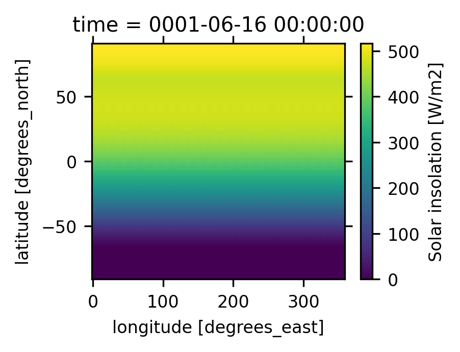
# Easier to find value for SNARL (37.6N, -118.8E)

ds_PI.SOLIN.isel(time=5).hvplot(coastline=True, cmap='viridis')
ds_PI.SOLIN
<xarray.DataArray 'SOLIN' (time: 12, lat: 96, lon: 144)> Size: 664kB
dask.array<concatenate, shape=(12, 96, 144), dtype=float32, chunksize=(1, 96, 144), chunktype=numpy.ndarray>
Coordinates:
  * time     (time) object 96B 0001-01-17 00:00:00 ... 0001-12-17 00:00:00
  * lat      (lat) float64 768B -90.0 -88.11 -86.21 -84.32 ... 86.21 88.11 90.0
  * lon      (lon) float64 1kB 0.0 2.5 5.0 7.5 10.0 ... 350.0 352.5 355.0 357.5
Attributes:
    Sampling_Sequence:  rad_lwsw
    units:              W/m2
    long_name:          Solar insolation
cell_methods: time: mean- time: 12
- lat: 96
- lon: 144
- dask.array<chunksize=(1, 96, 144), meta=np.ndarray>
Array Chunk Bytes 648.00 kiB 54.00 kiB Shape (12, 96, 144) (1, 96, 144) Dask graph 12 chunks in 25 graph layers Data type float32 numpy.ndarray - time(time)object0001-01-17 00:00:00 ... 0001-12-...
array([cftime.DatetimeNoLeap(1, 1, 17, 0, 0, 0, 0, has_year_zero=True), cftime.DatetimeNoLeap(1, 2, 14, 0, 0, 0, 0, has_year_zero=True), cftime.DatetimeNoLeap(1, 3, 17, 0, 0, 0, 0, has_year_zero=True), cftime.DatetimeNoLeap(1, 4, 16, 0, 0, 0, 0, has_year_zero=True), cftime.DatetimeNoLeap(1, 5, 17, 0, 0, 0, 0, has_year_zero=True), cftime.DatetimeNoLeap(1, 6, 16, 0, 0, 0, 0, has_year_zero=True), cftime.DatetimeNoLeap(1, 7, 17, 0, 0, 0, 0, has_year_zero=True), cftime.DatetimeNoLeap(1, 8, 17, 0, 0, 0, 0, has_year_zero=True), cftime.DatetimeNoLeap(1, 9, 16, 0, 0, 0, 0, has_year_zero=True), cftime.DatetimeNoLeap(1, 10, 17, 0, 0, 0, 0, has_year_zero=True), cftime.DatetimeNoLeap(1, 11, 16, 0, 0, 0, 0, has_year_zero=True), cftime.DatetimeNoLeap(1, 12, 17, 0, 0, 0, 0, has_year_zero=True)], dtype=object) - lat(lat)float64-90.0 -88.11 -86.21 ... 88.11 90.0
- long_name :
- latitude
- units :
- degrees_north
array([-90. , -88.105263, -86.210526, -84.315789, -82.421053, -80.526316, -78.631579, -76.736842, -74.842105, -72.947368, -71.052632, -69.157895, -67.263158, -65.368421, -63.473684, -61.578947, -59.684211, -57.789474, -55.894737, -54. , -52.105263, -50.210526, -48.315789, -46.421053, -44.526316, -42.631579, -40.736842, -38.842105, -36.947368, -35.052632, -33.157895, -31.263158, -29.368421, -27.473684, -25.578947, -23.684211, -21.789474, -19.894737, -18. , -16.105263, -14.210526, -12.315789, -10.421053, -8.526316, -6.631579, -4.736842, -2.842105, -0.947368, 0.947368, 2.842105, 4.736842, 6.631579, 8.526316, 10.421053, 12.315789, 14.210526, 16.105263, 18. , 19.894737, 21.789474, 23.684211, 25.578947, 27.473684, 29.368421, 31.263158, 33.157895, 35.052632, 36.947368, 38.842105, 40.736842, 42.631579, 44.526316, 46.421053, 48.315789, 50.210526, 52.105263, 54. , 55.894737, 57.789474, 59.684211, 61.578947, 63.473684, 65.368421, 67.263158, 69.157895, 71.052632, 72.947368, 74.842105, 76.736842, 78.631579, 80.526316, 82.421053, 84.315789, 86.210526, 88.105263, 90. ]) - lon(lon)float640.0 2.5 5.0 ... 352.5 355.0 357.5
- long_name :
- longitude
- units :
- degrees_east
array([  0. ,   2.5,   5. ,   7.5,  10. ,  12.5,  15. ,  17.5,  20. ,  22.5,
        25. ,  27.5,  30. ,  32.5,  35. ,  37.5,  40. ,  42.5,  45. ,  47.5,
        50. ,  52.5,  55. ,  57.5,  60. ,  62.5,  65. ,  67.5,  70. ,  72.5,
        75. ,  77.5,  80. ,  82.5,  85. ,  87.5,  90. ,  92.5,  95. ,  97.5,
       100. , 102.5, 105. , 107.5, 110. , 112.5, 115. , 117.5, 120. , 122.5,
       125. , 127.5, 130. , 132.5, 135. , 137.5, 140. , 142.5, 145. , 147.5,
       150. , 152.5, 155. , 157.5, 160. , 162.5, 165. , 167.5, 170. , 172.5,
       175. , 177.5, 180. , 182.5, 185. , 187.5, 190. , 192.5, 195. , 197.5,
       200. , 202.5, 205. , 207.5, 210. , 212.5, 215. , 217.5, 220. , 222.5,
       225. , 227.5, 230. , 232.5, 235. , 237.5, 240. , 242.5, 245. , 247.5,
       250. , 252.5, 255. , 257.5, 260. , 262.5, 265. , 267.5, 270. , 272.5,
       275. , 277.5, 280. , 282.5, 285. , 287.5, 290. , 292.5, 295. , 297.5,
       300. , 302.5, 305. , 307.5, 310. , 312.5, 315. , 317.5, 320. , 322.5,
       325. , 327.5, 330. , 332.5, 335. , 337.5, 340. , 342.5, 345. , 347.5,
       350. , 352.5, 355. , 357.5])
- Sampling_Sequence :
- rad_lwsw
- units :
- W/m2
- long_name :
- Solar insolation
- cell_methods :
- time: mean
# Compute zonal mean and make plot of piControl
ds_PI.SOLIN.mean('lon').plot.contourf(x='time', y='lat', figsize=(4, 2))
plt.xlabel('time (year-month)')
Text(0.5, 0, 'time (year-month)')
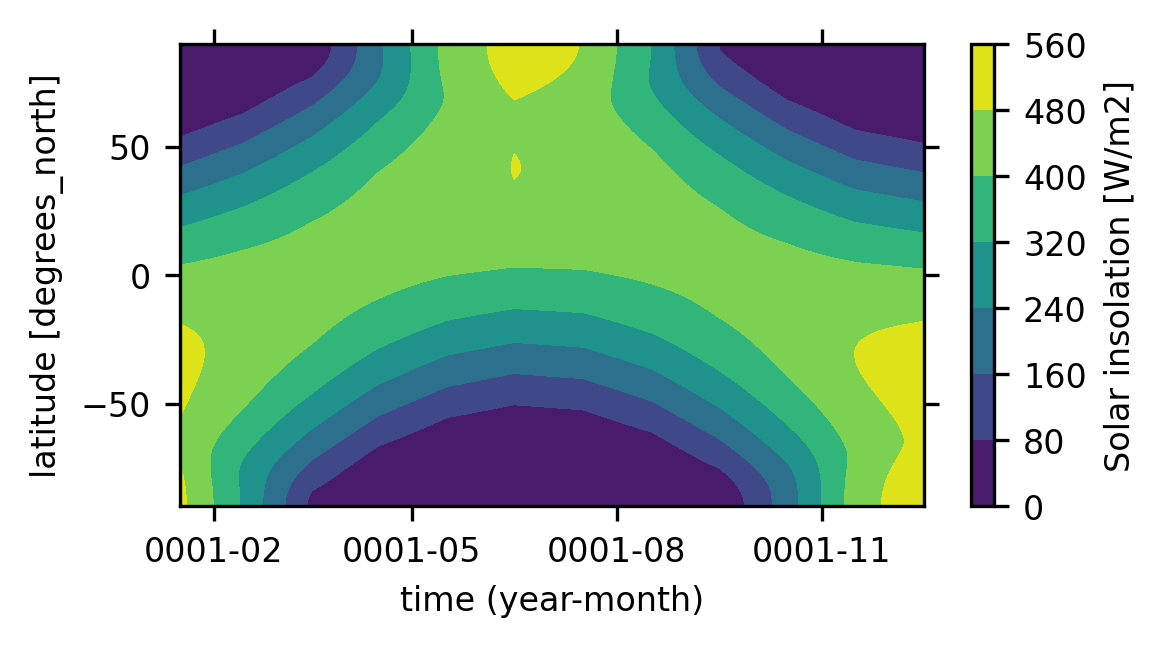
# Add your code to compute zonal mean and make plot of midHolocene
# Add your code to compute and plot the difference: midHolocen - piControl zonal mean
Click here for the solution
Copy and paste the code into the above cell
ds_MH.SOLIN.mean('lon').plot.contourf(x='time', y='lat', figsize=(4, 2))

(ds_MH.SOLIN - ds_PI.SOLIN).mean('lon').plot.contourf(
    x='time', y='lat', figsize=(4, 2), levels=np.linspace(-30, 30, 21))
Small group discussion#
Which orbital parameters are different at the middle Holocene (6ka BP)?
How does the orbital parameter impact the top-of-atmosphere shortwave radiation (solar insolation)?
Do the results look correct? You can compare your results with Figure 3b of Otto-Bliesner et al., (2017)
Analysis 2: Does the Earth receive more radiation during the mid-Holocene?#
We compute the global annual mean solar insolation to answer this question.
Importantly, we need to weight grid cells by their area (equivalent to cosine of latitude), using the
.weightedmethod
Note that lat is in degrees
ds_PI.lat
<xarray.DataArray 'lat' (lat: 96)> Size: 768B
array([-90.      , -88.105263, -86.210526, -84.315789, -82.421053, -80.526316,
       -78.631579, -76.736842, -74.842105, -72.947368, -71.052632, -69.157895,
       -67.263158, -65.368421, -63.473684, -61.578947, -59.684211, -57.789474,
       -55.894737, -54.      , -52.105263, -50.210526, -48.315789, -46.421053,
       -44.526316, -42.631579, -40.736842, -38.842105, -36.947368, -35.052632,
       -33.157895, -31.263158, -29.368421, -27.473684, -25.578947, -23.684211,
       -21.789474, -19.894737, -18.      , -16.105263, -14.210526, -12.315789,
       -10.421053,  -8.526316,  -6.631579,  -4.736842,  -2.842105,  -0.947368,
         0.947368,   2.842105,   4.736842,   6.631579,   8.526316,  10.421053,
        12.315789,  14.210526,  16.105263,  18.      ,  19.894737,  21.789474,
        23.684211,  25.578947,  27.473684,  29.368421,  31.263158,  33.157895,
        35.052632,  36.947368,  38.842105,  40.736842,  42.631579,  44.526316,
        46.421053,  48.315789,  50.210526,  52.105263,  54.      ,  55.894737,
        57.789474,  59.684211,  61.578947,  63.473684,  65.368421,  67.263158,
        69.157895,  71.052632,  72.947368,  74.842105,  76.736842,  78.631579,
        80.526316,  82.421053,  84.315789,  86.210526,  88.105263,  90.      ])
Coordinates:
  * lat      (lat) float64 768B -90.0 -88.11 -86.21 -84.32 ... 86.21 88.11 90.0
Attributes:
    long_name:  latitude
units: degrees_north- lat: 96
- -90.0 -88.11 -86.21 -84.32 -82.42 ... 82.42 84.32 86.21 88.11 90.0
array([-90. , -88.105263, -86.210526, -84.315789, -82.421053, -80.526316, -78.631579, -76.736842, -74.842105, -72.947368, -71.052632, -69.157895, -67.263158, -65.368421, -63.473684, -61.578947, -59.684211, -57.789474, -55.894737, -54. , -52.105263, -50.210526, -48.315789, -46.421053, -44.526316, -42.631579, -40.736842, -38.842105, -36.947368, -35.052632, -33.157895, -31.263158, -29.368421, -27.473684, -25.578947, -23.684211, -21.789474, -19.894737, -18. , -16.105263, -14.210526, -12.315789, -10.421053, -8.526316, -6.631579, -4.736842, -2.842105, -0.947368, 0.947368, 2.842105, 4.736842, 6.631579, 8.526316, 10.421053, 12.315789, 14.210526, 16.105263, 18. , 19.894737, 21.789474, 23.684211, 25.578947, 27.473684, 29.368421, 31.263158, 33.157895, 35.052632, 36.947368, 38.842105, 40.736842, 42.631579, 44.526316, 46.421053, 48.315789, 50.210526, 52.105263, 54. , 55.894737, 57.789474, 59.684211, 61.578947, 63.473684, 65.368421, 67.263158, 69.157895, 71.052632, 72.947368, 74.842105, 76.736842, 78.631579, 80.526316, 82.421053, 84.315789, 86.210526, 88.105263, 90. ]) - lat(lat)float64-90.0 -88.11 -86.21 ... 88.11 90.0
- long_name :
- latitude
- units :
- degrees_north
array([-90.      , -88.105263, -86.210526, -84.315789, -82.421053, -80.526316,
       -78.631579, -76.736842, -74.842105, -72.947368, -71.052632, -69.157895,
       -67.263158, -65.368421, -63.473684, -61.578947, -59.684211, -57.789474,
       -55.894737, -54.      , -52.105263, -50.210526, -48.315789, -46.421053,
       -44.526316, -42.631579, -40.736842, -38.842105, -36.947368, -35.052632,
       -33.157895, -31.263158, -29.368421, -27.473684, -25.578947, -23.684211,
       -21.789474, -19.894737, -18.      , -16.105263, -14.210526, -12.315789,
       -10.421053,  -8.526316,  -6.631579,  -4.736842,  -2.842105,  -0.947368,
         0.947368,   2.842105,   4.736842,   6.631579,   8.526316,  10.421053,
        12.315789,  14.210526,  16.105263,  18.      ,  19.894737,  21.789474,
        23.684211,  25.578947,  27.473684,  29.368421,  31.263158,  33.157895,
        35.052632,  36.947368,  38.842105,  40.736842,  42.631579,  44.526316,
        46.421053,  48.315789,  50.210526,  52.105263,  54.      ,  55.894737,
        57.789474,  59.684211,  61.578947,  63.473684,  65.368421,  67.263158,
        69.157895,  71.052632,  72.947368,  74.842105,  76.736842,  78.631579,
        80.526316,  82.421053,  84.315789,  86.210526,  88.105263,  90.      ])
- long_name :
- latitude
- units :
- degrees_north
Example calculation for the piControl#
coslat = np.cos(np.deg2rad(ds_PI.lat))

SOLIN_PI = ds_PI.SOLIN.weighted(coslat).mean(('lat', 'lon', 'time'))

print("The global annual mean insolation of PI: ", SOLIN_PI.values, "W/m2")
The global annual mean insolation of PI: 340.32719678192876 W/m2
If we don’t apply the area weights, we will get a wrong answer#
SOLIN_PI_unweighted = ds_PI.SOLIN.mean(('lat', 'lon', 'time'))

print("Only if we forgot to properly weight the values by area (cosine(latitude)):",
      SOLIN_PI_unweighted.values, "W/m2")
Only if we forgot to properly weight the values by area (cosine(latitude)): 297.03168 W/m2
Add your own calculation for the midHolocene and compute the difference between midHolocene and piControl#
SOLIN_MH = ?
SOLIN_MH - SOLIN_PI = ?
Click here for the solution
Copy and paste the code into the above cellcoslat = np.cos(np.deg2rad(ds_MH.lat))
SOLIN_MH = ds_MH.SOLIN.weighted(coslat).mean(('lat', 'lon', 'time'))
print("The global annual mean insolation of MH: ", SOLIN_MH.values, "W/m2")
print("Difference, MH - PI: ", SOLIN_MH.values-SOLIN_PI.values, "W/m2")
Small group discussion#
Jess taught us in her lecture that obliquity and precession do not impact the global annual mean solar insolation, but why do we see different value in our midHolonece?
Click here for the solution
The code below should produce a larger value for midHolocene by ~0.012 W m-2 (0.004%).
The larger solar insolation is very likely due to the higher eccentricity in midHolocene (0.018682 vs 0.01676429)!
coslat = np.cos(np.deg2rad(ds_MH.lat))
month_length = ds_MH.time.dt.days_in_month

SOLIN_PI = ds_PI.SOLIN.weighted(month_length * coslat).mean(('time', 'lat', 'lon'))
SOLIN_MH = ds_MH.SOLIN.weighted(month_length * coslat).mean(('time', 'lat', 'lon'))

print("The global annual mean insolation of PI: ", SOLIN_PI.values, "W/m2")
print("The global annual mean insolation of MH: ", SOLIN_MH.values, "W/m2")
print("Difference, MH - PI: ", SOLIN_MH.values - SOLIN_PI.values, "W/m2")
Small group discussion#
Should the mid-Holocene be warmer or colder than the preindustrial (given that difference in solar insolation is only 0.012 W m-2, 0.004%)?
Holocene Temperature Conundrum: geological records suggest that mid-Holocene was warmer by ~0.5℃ than the preindustrial, while climate models suggest a colder mid-Holocene by ~0.5℃.
Why? Are models missing anything?
See one of the hypotheses in
4b_opt2_analyze_long_midHolocene.
Further reading: Liu et al. (2014); Osman et al. (2021)
Analysis 3: how does orbital forcing impact the ITCZ and monsoon precipitation during the midHolocene?#
In CESM, total precipitation is computed as
prec = PRECC + PRECL(sum of convective and large-scale precipitation; recall that climate models have to parameterize convection!)We convert the units from m/s into mm/day
We use
.isel(time=slice(5, 8))to select the June, July, and August values (recall that Python uses 0-based ordering)Let’s use Cartopy and Matplotlib with a Robinson projection (instead of using the simple Xarray.plot())
We use
add_cyclic_pointto get rid of the “white strip” in the plot
ds_PI.PRECC
<xarray.DataArray 'PRECC' (time: 12, lat: 96, lon: 144)> Size: 664kB
dask.array<concatenate, shape=(12, 96, 144), dtype=float32, chunksize=(1, 96, 144), chunktype=numpy.ndarray>
Coordinates:
  * time     (time) object 96B 0001-01-17 00:00:00 ... 0001-12-17 00:00:00
  * lat      (lat) float64 768B -90.0 -88.11 -86.21 -84.32 ... 86.21 88.11 90.0
  * lon      (lon) float64 1kB 0.0 2.5 5.0 7.5 10.0 ... 350.0 352.5 355.0 357.5
Attributes:
    units:         m/s
    long_name:     Convective precipitation rate (liq + ice)
cell_methods: time: mean- time: 12
- lat: 96
- lon: 144
- dask.array<chunksize=(1, 96, 144), meta=np.ndarray>
Array Chunk Bytes 648.00 kiB 54.00 kiB Shape (12, 96, 144) (1, 96, 144) Dask graph 12 chunks in 25 graph layers Data type float32 numpy.ndarray - time(time)object0001-01-17 00:00:00 ... 0001-12-...
array([cftime.DatetimeNoLeap(1, 1, 17, 0, 0, 0, 0, has_year_zero=True), cftime.DatetimeNoLeap(1, 2, 14, 0, 0, 0, 0, has_year_zero=True), cftime.DatetimeNoLeap(1, 3, 17, 0, 0, 0, 0, has_year_zero=True), cftime.DatetimeNoLeap(1, 4, 16, 0, 0, 0, 0, has_year_zero=True), cftime.DatetimeNoLeap(1, 5, 17, 0, 0, 0, 0, has_year_zero=True), cftime.DatetimeNoLeap(1, 6, 16, 0, 0, 0, 0, has_year_zero=True), cftime.DatetimeNoLeap(1, 7, 17, 0, 0, 0, 0, has_year_zero=True), cftime.DatetimeNoLeap(1, 8, 17, 0, 0, 0, 0, has_year_zero=True), cftime.DatetimeNoLeap(1, 9, 16, 0, 0, 0, 0, has_year_zero=True), cftime.DatetimeNoLeap(1, 10, 17, 0, 0, 0, 0, has_year_zero=True), cftime.DatetimeNoLeap(1, 11, 16, 0, 0, 0, 0, has_year_zero=True), cftime.DatetimeNoLeap(1, 12, 17, 0, 0, 0, 0, has_year_zero=True)], dtype=object) - lat(lat)float64-90.0 -88.11 -86.21 ... 88.11 90.0
- long_name :
- latitude
- units :
- degrees_north
array([-90. , -88.105263, -86.210526, -84.315789, -82.421053, -80.526316, -78.631579, -76.736842, -74.842105, -72.947368, -71.052632, -69.157895, -67.263158, -65.368421, -63.473684, -61.578947, -59.684211, -57.789474, -55.894737, -54. , -52.105263, -50.210526, -48.315789, -46.421053, -44.526316, -42.631579, -40.736842, -38.842105, -36.947368, -35.052632, -33.157895, -31.263158, -29.368421, -27.473684, -25.578947, -23.684211, -21.789474, -19.894737, -18. , -16.105263, -14.210526, -12.315789, -10.421053, -8.526316, -6.631579, -4.736842, -2.842105, -0.947368, 0.947368, 2.842105, 4.736842, 6.631579, 8.526316, 10.421053, 12.315789, 14.210526, 16.105263, 18. , 19.894737, 21.789474, 23.684211, 25.578947, 27.473684, 29.368421, 31.263158, 33.157895, 35.052632, 36.947368, 38.842105, 40.736842, 42.631579, 44.526316, 46.421053, 48.315789, 50.210526, 52.105263, 54. , 55.894737, 57.789474, 59.684211, 61.578947, 63.473684, 65.368421, 67.263158, 69.157895, 71.052632, 72.947368, 74.842105, 76.736842, 78.631579, 80.526316, 82.421053, 84.315789, 86.210526, 88.105263, 90. ]) - lon(lon)float640.0 2.5 5.0 ... 352.5 355.0 357.5
- long_name :
- longitude
- units :
- degrees_east
array([  0. ,   2.5,   5. ,   7.5,  10. ,  12.5,  15. ,  17.5,  20. ,  22.5,
        25. ,  27.5,  30. ,  32.5,  35. ,  37.5,  40. ,  42.5,  45. ,  47.5,
        50. ,  52.5,  55. ,  57.5,  60. ,  62.5,  65. ,  67.5,  70. ,  72.5,
        75. ,  77.5,  80. ,  82.5,  85. ,  87.5,  90. ,  92.5,  95. ,  97.5,
       100. , 102.5, 105. , 107.5, 110. , 112.5, 115. , 117.5, 120. , 122.5,
       125. , 127.5, 130. , 132.5, 135. , 137.5, 140. , 142.5, 145. , 147.5,
       150. , 152.5, 155. , 157.5, 160. , 162.5, 165. , 167.5, 170. , 172.5,
       175. , 177.5, 180. , 182.5, 185. , 187.5, 190. , 192.5, 195. , 197.5,
       200. , 202.5, 205. , 207.5, 210. , 212.5, 215. , 217.5, 220. , 222.5,
       225. , 227.5, 230. , 232.5, 235. , 237.5, 240. , 242.5, 245. , 247.5,
       250. , 252.5, 255. , 257.5, 260. , 262.5, 265. , 267.5, 270. , 272.5,
       275. , 277.5, 280. , 282.5, 285. , 287.5, 290. , 292.5, 295. , 297.5,
       300. , 302.5, 305. , 307.5, 310. , 312.5, 315. , 317.5, 320. , 322.5,
       325. , 327.5, 330. , 332.5, 335. , 337.5, 340. , 342.5, 345. , 347.5,
       350. , 352.5, 355. , 357.5])
- units :
- m/s
- long_name :
- Convective precipitation rate (liq + ice)
- cell_methods :
- time: mean
ds_PI.PRECL
<xarray.DataArray 'PRECL' (time: 12, lat: 96, lon: 144)> Size: 664kB
dask.array<concatenate, shape=(12, 96, 144), dtype=float32, chunksize=(1, 96, 144), chunktype=numpy.ndarray>
Coordinates:
  * time     (time) object 96B 0001-01-17 00:00:00 ... 0001-12-17 00:00:00
  * lat      (lat) float64 768B -90.0 -88.11 -86.21 -84.32 ... 86.21 88.11 90.0
  * lon      (lon) float64 1kB 0.0 2.5 5.0 7.5 10.0 ... 350.0 352.5 355.0 357.5
Attributes:
    units:         m/s
    long_name:     Large-scale (stable) precipitation rate (liq + ice)
cell_methods: time: mean- time: 12
- lat: 96
- lon: 144
- dask.array<chunksize=(1, 96, 144), meta=np.ndarray>
Array Chunk Bytes 648.00 kiB 54.00 kiB Shape (12, 96, 144) (1, 96, 144) Dask graph 12 chunks in 25 graph layers Data type float32 numpy.ndarray - time(time)object0001-01-17 00:00:00 ... 0001-12-...
array([cftime.DatetimeNoLeap(1, 1, 17, 0, 0, 0, 0, has_year_zero=True), cftime.DatetimeNoLeap(1, 2, 14, 0, 0, 0, 0, has_year_zero=True), cftime.DatetimeNoLeap(1, 3, 17, 0, 0, 0, 0, has_year_zero=True), cftime.DatetimeNoLeap(1, 4, 16, 0, 0, 0, 0, has_year_zero=True), cftime.DatetimeNoLeap(1, 5, 17, 0, 0, 0, 0, has_year_zero=True), cftime.DatetimeNoLeap(1, 6, 16, 0, 0, 0, 0, has_year_zero=True), cftime.DatetimeNoLeap(1, 7, 17, 0, 0, 0, 0, has_year_zero=True), cftime.DatetimeNoLeap(1, 8, 17, 0, 0, 0, 0, has_year_zero=True), cftime.DatetimeNoLeap(1, 9, 16, 0, 0, 0, 0, has_year_zero=True), cftime.DatetimeNoLeap(1, 10, 17, 0, 0, 0, 0, has_year_zero=True), cftime.DatetimeNoLeap(1, 11, 16, 0, 0, 0, 0, has_year_zero=True), cftime.DatetimeNoLeap(1, 12, 17, 0, 0, 0, 0, has_year_zero=True)], dtype=object) - lat(lat)float64-90.0 -88.11 -86.21 ... 88.11 90.0
- long_name :
- latitude
- units :
- degrees_north
array([-90. , -88.105263, -86.210526, -84.315789, -82.421053, -80.526316, -78.631579, -76.736842, -74.842105, -72.947368, -71.052632, -69.157895, -67.263158, -65.368421, -63.473684, -61.578947, -59.684211, -57.789474, -55.894737, -54. , -52.105263, -50.210526, -48.315789, -46.421053, -44.526316, -42.631579, -40.736842, -38.842105, -36.947368, -35.052632, -33.157895, -31.263158, -29.368421, -27.473684, -25.578947, -23.684211, -21.789474, -19.894737, -18. , -16.105263, -14.210526, -12.315789, -10.421053, -8.526316, -6.631579, -4.736842, -2.842105, -0.947368, 0.947368, 2.842105, 4.736842, 6.631579, 8.526316, 10.421053, 12.315789, 14.210526, 16.105263, 18. , 19.894737, 21.789474, 23.684211, 25.578947, 27.473684, 29.368421, 31.263158, 33.157895, 35.052632, 36.947368, 38.842105, 40.736842, 42.631579, 44.526316, 46.421053, 48.315789, 50.210526, 52.105263, 54. , 55.894737, 57.789474, 59.684211, 61.578947, 63.473684, 65.368421, 67.263158, 69.157895, 71.052632, 72.947368, 74.842105, 76.736842, 78.631579, 80.526316, 82.421053, 84.315789, 86.210526, 88.105263, 90. ]) - lon(lon)float640.0 2.5 5.0 ... 352.5 355.0 357.5
- long_name :
- longitude
- units :
- degrees_east
array([  0. ,   2.5,   5. ,   7.5,  10. ,  12.5,  15. ,  17.5,  20. ,  22.5,
        25. ,  27.5,  30. ,  32.5,  35. ,  37.5,  40. ,  42.5,  45. ,  47.5,
        50. ,  52.5,  55. ,  57.5,  60. ,  62.5,  65. ,  67.5,  70. ,  72.5,
        75. ,  77.5,  80. ,  82.5,  85. ,  87.5,  90. ,  92.5,  95. ,  97.5,
       100. , 102.5, 105. , 107.5, 110. , 112.5, 115. , 117.5, 120. , 122.5,
       125. , 127.5, 130. , 132.5, 135. , 137.5, 140. , 142.5, 145. , 147.5,
       150. , 152.5, 155. , 157.5, 160. , 162.5, 165. , 167.5, 170. , 172.5,
       175. , 177.5, 180. , 182.5, 185. , 187.5, 190. , 192.5, 195. , 197.5,
       200. , 202.5, 205. , 207.5, 210. , 212.5, 215. , 217.5, 220. , 222.5,
       225. , 227.5, 230. , 232.5, 235. , 237.5, 240. , 242.5, 245. , 247.5,
       250. , 252.5, 255. , 257.5, 260. , 262.5, 265. , 267.5, 270. , 272.5,
       275. , 277.5, 280. , 282.5, 285. , 287.5, 290. , 292.5, 295. , 297.5,
       300. , 302.5, 305. , 307.5, 310. , 312.5, 315. , 317.5, 320. , 322.5,
       325. , 327.5, 330. , 332.5, 335. , 337.5, 340. , 342.5, 345. , 347.5,
       350. , 352.5, 355. , 357.5])
- units :
- m/s
- long_name :
- Large-scale (stable) precipitation rate (liq + ice)
- cell_methods :
- time: mean
m_p_s_to_mm_p_day = 86400 * 1000

prec_PI = (ds_PI.PRECC + ds_PI.PRECL).isel(time=slice(5, 8)).mean('time') * m_p_s_to_mm_p_day

prec_MH = (ds_MH.PRECC + ds_MH.PRECL).isel(time=slice(5, 8)).mean('time') * m_p_s_to_mm_p_day

prec_PI
<xarray.DataArray (lat: 96, lon: 144)> Size: 55kB
dask.array<mul, shape=(96, 144), dtype=float32, chunksize=(96, 144), chunktype=numpy.ndarray>
Coordinates:
  * lat      (lat) float64 768B -90.0 -88.11 -86.21 -84.32 ... 86.21 88.11 90.0
  * lon      (lon) float64 1kB 0.0 2.5 5.0 7.5 10.0 ... 350.0 352.5 355.0 357.5
Attributes:
    units:         m/s
cell_methods: time: mean- lat: 96
- lon: 144
- dask.array<chunksize=(96, 144), meta=np.ndarray>
Array Chunk Bytes 54.00 kiB 54.00 kiB Shape (96, 144) (96, 144) Dask graph 1 chunks in 55 graph layers Data type float32 numpy.ndarray - lat(lat)float64-90.0 -88.11 -86.21 ... 88.11 90.0
- long_name :
- latitude
- units :
- degrees_north
array([-90. , -88.105263, -86.210526, -84.315789, -82.421053, -80.526316, -78.631579, -76.736842, -74.842105, -72.947368, -71.052632, -69.157895, -67.263158, -65.368421, -63.473684, -61.578947, -59.684211, -57.789474, -55.894737, -54. , -52.105263, -50.210526, -48.315789, -46.421053, -44.526316, -42.631579, -40.736842, -38.842105, -36.947368, -35.052632, -33.157895, -31.263158, -29.368421, -27.473684, -25.578947, -23.684211, -21.789474, -19.894737, -18. , -16.105263, -14.210526, -12.315789, -10.421053, -8.526316, -6.631579, -4.736842, -2.842105, -0.947368, 0.947368, 2.842105, 4.736842, 6.631579, 8.526316, 10.421053, 12.315789, 14.210526, 16.105263, 18. , 19.894737, 21.789474, 23.684211, 25.578947, 27.473684, 29.368421, 31.263158, 33.157895, 35.052632, 36.947368, 38.842105, 40.736842, 42.631579, 44.526316, 46.421053, 48.315789, 50.210526, 52.105263, 54. , 55.894737, 57.789474, 59.684211, 61.578947, 63.473684, 65.368421, 67.263158, 69.157895, 71.052632, 72.947368, 74.842105, 76.736842, 78.631579, 80.526316, 82.421053, 84.315789, 86.210526, 88.105263, 90. ]) - lon(lon)float640.0 2.5 5.0 ... 352.5 355.0 357.5
- long_name :
- longitude
- units :
- degrees_east
array([  0. ,   2.5,   5. ,   7.5,  10. ,  12.5,  15. ,  17.5,  20. ,  22.5,
        25. ,  27.5,  30. ,  32.5,  35. ,  37.5,  40. ,  42.5,  45. ,  47.5,
        50. ,  52.5,  55. ,  57.5,  60. ,  62.5,  65. ,  67.5,  70. ,  72.5,
        75. ,  77.5,  80. ,  82.5,  85. ,  87.5,  90. ,  92.5,  95. ,  97.5,
       100. , 102.5, 105. , 107.5, 110. , 112.5, 115. , 117.5, 120. , 122.5,
       125. , 127.5, 130. , 132.5, 135. , 137.5, 140. , 142.5, 145. , 147.5,
       150. , 152.5, 155. , 157.5, 160. , 162.5, 165. , 167.5, 170. , 172.5,
       175. , 177.5, 180. , 182.5, 185. , 187.5, 190. , 192.5, 195. , 197.5,
       200. , 202.5, 205. , 207.5, 210. , 212.5, 215. , 217.5, 220. , 222.5,
       225. , 227.5, 230. , 232.5, 235. , 237.5, 240. , 242.5, 245. , 247.5,
       250. , 252.5, 255. , 257.5, 260. , 262.5, 265. , 267.5, 270. , 272.5,
       275. , 277.5, 280. , 282.5, 285. , 287.5, 290. , 292.5, 295. , 297.5,
       300. , 302.5, 305. , 307.5, 310. , 312.5, 315. , 317.5, 320. , 322.5,
       325. , 327.5, 330. , 332.5, 335. , 337.5, 340. , 342.5, 345. , 347.5,
       350. , 352.5, 355. , 357.5])
- units :
- m/s
- cell_methods :
- time: mean
Plot total precipitation of piControl#
fig, ax = plt.subplots(figsize=(3, 1.5), subplot_kw={
    'projection': ccrs.Robinson(central_longitude=210)})

p1 = ax.contourf(prec_PI.lon, prec_PI.lat, prec_PI,
                 cmap='YlGnBu',
                 levels=np.linspace(0, 17, 18),
                 extend='both',
                 transform=ccrs.PlateCarree())

ax.coastlines(linewidth=0.5)
plt.colorbar(p1)
ax.set_title("PI precipitation")
Text(0.5, 1.0, 'PI precipitation')
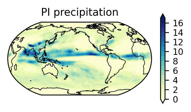
Let’s use add_cyclic_point to get rid of the “white strip” in the plot#
fig, ax = plt.subplots(figsize=(3, 1.5), subplot_kw={
    'projection': ccrs.Robinson(central_longitude=210)})

# Note the differences in the next two lines
prec_PI_new, lon_new = add_cyclic_point(prec_PI, prec_PI.lon)
p1 = ax.contourf(lon_new, prec_PI.lat, prec_PI_new,
                 cmap='YlGnBu',
                 levels=np.linspace(0, 17, 18),
                 extend='both',
                 transform=ccrs.PlateCarree())

ax.coastlines(linewidth=0.5)
plt.colorbar(p1)
ax.set_title("PI precipitation")
Text(0.5, 1.0, 'PI precipitation')
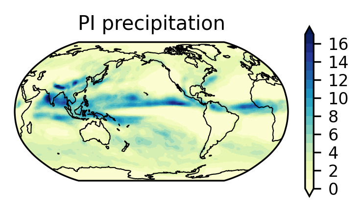
Add your own plot of the midHolocene precipitation#
fig, ax = plt.subplots(figsize=(3, 1.5), subplot_kw={
    'projection': ccrs.Robinson(central_longitude=210)})

Add your own plot of the midHolocene - piControl#
fig, ax = plt.subplots(figsize=(3, 1.5), subplot_kw={
    'projection': ccrs.Robinson(central_longitude=210)})
Click here for the solution
Copy and paste the code into the above cellprec_MH_new, lon_new = add_cyclic_point(prec_MH, prec_MH.lon)
p1 = ax.contourf(lon_new, prec_MH.lat, prec_MH_new,
cmap='YlGnBu',
levels=np.linspace(0, 17, 18),
extend='both',
transform=ccrs.PlateCarree())
ax.coastlines(linewidth=0.5)
plt.colorbar(p1)
ax.set_title("MH precipitation")
p1 = ax.contourf(lon_new, prec_MH.lat, prec_MH_new - prec_PI_new,
                 cmap='BrBG',
                 levels=np.linspace(-5, 5, 21),
                 extend='both',
                 transform=ccrs.PlateCarree())

ax.coastlines(linewidth=0.5)
plt.colorbar(p1)
ax.set_title("MH precipitation anomalies")
Discussion#
Do you see the ITCZ in the piControl?
How does the ITCZ change in the mid-Holocene?
Do you see changes of the monsoon precipitation? Is it consistent with findings from Kutzbach and Otto-Bliesner (1981, 1982)?
Ask the instructors about ITCZ and monsoon!
Analysis 4: how does the MH orbital forcing impact the atmospheric circulation?#
We plot the zonal mean zonal wind of PI in the Northern Hemisphere summer (JJA)
We use
plt.gca().invert_yaxis()to invert the y-axis such that the high pressure is at the bottom
ds_PI.U
<xarray.DataArray 'U' (time: 12, lev: 26, lat: 96, lon: 144)> Size: 17MB
dask.array<concatenate, shape=(12, 26, 96, 144), dtype=float32, chunksize=(1, 26, 96, 144), chunktype=numpy.ndarray>
Coordinates:
  * time     (time) object 96B 0001-01-17 00:00:00 ... 0001-12-17 00:00:00
  * lev      (lev) float64 208B 3.545 7.389 13.97 23.94 ... 929.6 970.6 992.6
  * lat      (lat) float64 768B -90.0 -88.11 -86.21 -84.32 ... 86.21 88.11 90.0
  * lon      (lon) float64 1kB 0.0 2.5 5.0 7.5 10.0 ... 350.0 352.5 355.0 357.5
Attributes:
    mdims:         1
    units:         m/s
    long_name:     Zonal wind
cell_methods: time: mean- time: 12
- lev: 26
- lat: 96
- lon: 144
- dask.array<chunksize=(1, 26, 96, 144), meta=np.ndarray>
Array Chunk Bytes 16.45 MiB 1.37 MiB Shape (12, 26, 96, 144) (1, 26, 96, 144) Dask graph 12 chunks in 25 graph layers Data type float32 numpy.ndarray - time(time)object0001-01-17 00:00:00 ... 0001-12-...
array([cftime.DatetimeNoLeap(1, 1, 17, 0, 0, 0, 0, has_year_zero=True), cftime.DatetimeNoLeap(1, 2, 14, 0, 0, 0, 0, has_year_zero=True), cftime.DatetimeNoLeap(1, 3, 17, 0, 0, 0, 0, has_year_zero=True), cftime.DatetimeNoLeap(1, 4, 16, 0, 0, 0, 0, has_year_zero=True), cftime.DatetimeNoLeap(1, 5, 17, 0, 0, 0, 0, has_year_zero=True), cftime.DatetimeNoLeap(1, 6, 16, 0, 0, 0, 0, has_year_zero=True), cftime.DatetimeNoLeap(1, 7, 17, 0, 0, 0, 0, has_year_zero=True), cftime.DatetimeNoLeap(1, 8, 17, 0, 0, 0, 0, has_year_zero=True), cftime.DatetimeNoLeap(1, 9, 16, 0, 0, 0, 0, has_year_zero=True), cftime.DatetimeNoLeap(1, 10, 17, 0, 0, 0, 0, has_year_zero=True), cftime.DatetimeNoLeap(1, 11, 16, 0, 0, 0, 0, has_year_zero=True), cftime.DatetimeNoLeap(1, 12, 17, 0, 0, 0, 0, has_year_zero=True)], dtype=object) - lev(lev)float643.545 7.389 13.97 ... 970.6 992.6
- long_name :
- hybrid level at midpoints (1000*(A+B))
- units :
- hPa
- positive :
- down
- standard_name :
- atmosphere_hybrid_sigma_pressure_coordinate
- formula_terms :
- a: hyam b: hybm p0: P0 ps: PS
array([ 3.544638, 7.388814, 13.967214, 23.944625, 37.23029 , 53.114605, 70.05915 , 85.439115, 100.514695, 118.250335, 139.115395, 163.66207 , 192.539935, 226.513265, 266.481155, 313.501265, 368.81798 , 433.895225, 510.455255, 600.5242 , 696.79629 , 787.70206 , 867.16076 , 929.648875, 970.55483 , 992.5561 ]) - lat(lat)float64-90.0 -88.11 -86.21 ... 88.11 90.0
- long_name :
- latitude
- units :
- degrees_north
array([-90. , -88.105263, -86.210526, -84.315789, -82.421053, -80.526316, -78.631579, -76.736842, -74.842105, -72.947368, -71.052632, -69.157895, -67.263158, -65.368421, -63.473684, -61.578947, -59.684211, -57.789474, -55.894737, -54. , -52.105263, -50.210526, -48.315789, -46.421053, -44.526316, -42.631579, -40.736842, -38.842105, -36.947368, -35.052632, -33.157895, -31.263158, -29.368421, -27.473684, -25.578947, -23.684211, -21.789474, -19.894737, -18. , -16.105263, -14.210526, -12.315789, -10.421053, -8.526316, -6.631579, -4.736842, -2.842105, -0.947368, 0.947368, 2.842105, 4.736842, 6.631579, 8.526316, 10.421053, 12.315789, 14.210526, 16.105263, 18. , 19.894737, 21.789474, 23.684211, 25.578947, 27.473684, 29.368421, 31.263158, 33.157895, 35.052632, 36.947368, 38.842105, 40.736842, 42.631579, 44.526316, 46.421053, 48.315789, 50.210526, 52.105263, 54. , 55.894737, 57.789474, 59.684211, 61.578947, 63.473684, 65.368421, 67.263158, 69.157895, 71.052632, 72.947368, 74.842105, 76.736842, 78.631579, 80.526316, 82.421053, 84.315789, 86.210526, 88.105263, 90. ]) - lon(lon)float640.0 2.5 5.0 ... 352.5 355.0 357.5
- long_name :
- longitude
- units :
- degrees_east
array([  0. ,   2.5,   5. ,   7.5,  10. ,  12.5,  15. ,  17.5,  20. ,  22.5,
        25. ,  27.5,  30. ,  32.5,  35. ,  37.5,  40. ,  42.5,  45. ,  47.5,
        50. ,  52.5,  55. ,  57.5,  60. ,  62.5,  65. ,  67.5,  70. ,  72.5,
        75. ,  77.5,  80. ,  82.5,  85. ,  87.5,  90. ,  92.5,  95. ,  97.5,
       100. , 102.5, 105. , 107.5, 110. , 112.5, 115. , 117.5, 120. , 122.5,
       125. , 127.5, 130. , 132.5, 135. , 137.5, 140. , 142.5, 145. , 147.5,
       150. , 152.5, 155. , 157.5, 160. , 162.5, 165. , 167.5, 170. , 172.5,
       175. , 177.5, 180. , 182.5, 185. , 187.5, 190. , 192.5, 195. , 197.5,
       200. , 202.5, 205. , 207.5, 210. , 212.5, 215. , 217.5, 220. , 222.5,
       225. , 227.5, 230. , 232.5, 235. , 237.5, 240. , 242.5, 245. , 247.5,
       250. , 252.5, 255. , 257.5, 260. , 262.5, 265. , 267.5, 270. , 272.5,
       275. , 277.5, 280. , 282.5, 285. , 287.5, 290. , 292.5, 295. , 297.5,
       300. , 302.5, 305. , 307.5, 310. , 312.5, 315. , 317.5, 320. , 322.5,
       325. , 327.5, 330. , 332.5, 335. , 337.5, 340. , 342.5, 345. , 347.5,
       350. , 352.5, 355. , 357.5])
- mdims :
- 1
- units :
- m/s
- long_name :
- Zonal wind
- cell_methods :
- time: mean
Plot the zonal mean of u-winds of JJA#
U_PI_za_jja = ds_PI.U.isel(time=slice(5, 8)).mean(('lon', 'time'))

U_PI_za_jja.plot.contourf(figsize=(3, 1.5),
                          levels=np.linspace(-50, 50, 21), extend='both', )
plt.gca().invert_yaxis()
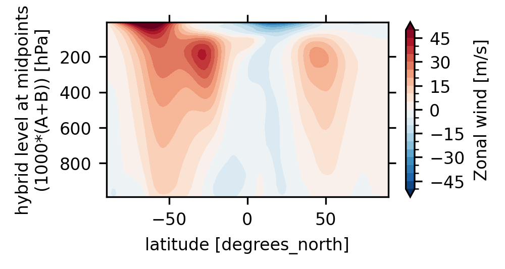
Add your own plot to show the changes during the midHolocene#
Click here for the solution
Copy and paste the code into the above cell
dU_MH_za_jja = (ds_MH.U - ds_PI.U).isel(time=slice(5, 8)).mean(('lon', 'time'))

dU_MH_za_jja.plot.contourf(figsize=(3, 1.5),
                          levels=np.linspace(-10, 10, 21), extend='both', )
plt.gca().invert_yaxis()
Did you notice any problem with the above plots?#
Check out the name of the vertical levels. It is called the hybrid sigma-pressure coordinate, which is NOT the pressure coordinate.
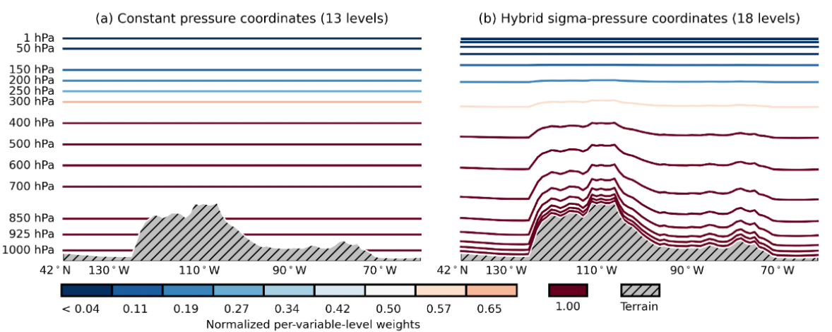
Figure: Atmosphere vertical coordinates
We need to interpolate from the hybrid sigma-pressure coordinate into the normal pressure coordinate
ds_PI.lev.standard_name
'atmosphere_hybrid_sigma_pressure_coordinate'
Use geocat interpolation to interpolate from hybrid sigma-pressure to pressure coordinate#
ds_PI.U
<xarray.DataArray 'U' (time: 12, lev: 26, lat: 96, lon: 144)> Size: 17MB
dask.array<concatenate, shape=(12, 26, 96, 144), dtype=float32, chunksize=(1, 26, 96, 144), chunktype=numpy.ndarray>
Coordinates:
  * time     (time) object 96B 0001-01-17 00:00:00 ... 0001-12-17 00:00:00
  * lev      (lev) float64 208B 3.545 7.389 13.97 23.94 ... 929.6 970.6 992.6
  * lat      (lat) float64 768B -90.0 -88.11 -86.21 -84.32 ... 86.21 88.11 90.0
  * lon      (lon) float64 1kB 0.0 2.5 5.0 7.5 10.0 ... 350.0 352.5 355.0 357.5
Attributes:
    mdims:         1
    units:         m/s
    long_name:     Zonal wind
cell_methods: time: mean- time: 12
- lev: 26
- lat: 96
- lon: 144
- dask.array<chunksize=(1, 26, 96, 144), meta=np.ndarray>
Array Chunk Bytes 16.45 MiB 1.37 MiB Shape (12, 26, 96, 144) (1, 26, 96, 144) Dask graph 12 chunks in 25 graph layers Data type float32 numpy.ndarray - time(time)object0001-01-17 00:00:00 ... 0001-12-...
array([cftime.DatetimeNoLeap(1, 1, 17, 0, 0, 0, 0, has_year_zero=True), cftime.DatetimeNoLeap(1, 2, 14, 0, 0, 0, 0, has_year_zero=True), cftime.DatetimeNoLeap(1, 3, 17, 0, 0, 0, 0, has_year_zero=True), cftime.DatetimeNoLeap(1, 4, 16, 0, 0, 0, 0, has_year_zero=True), cftime.DatetimeNoLeap(1, 5, 17, 0, 0, 0, 0, has_year_zero=True), cftime.DatetimeNoLeap(1, 6, 16, 0, 0, 0, 0, has_year_zero=True), cftime.DatetimeNoLeap(1, 7, 17, 0, 0, 0, 0, has_year_zero=True), cftime.DatetimeNoLeap(1, 8, 17, 0, 0, 0, 0, has_year_zero=True), cftime.DatetimeNoLeap(1, 9, 16, 0, 0, 0, 0, has_year_zero=True), cftime.DatetimeNoLeap(1, 10, 17, 0, 0, 0, 0, has_year_zero=True), cftime.DatetimeNoLeap(1, 11, 16, 0, 0, 0, 0, has_year_zero=True), cftime.DatetimeNoLeap(1, 12, 17, 0, 0, 0, 0, has_year_zero=True)], dtype=object) - lev(lev)float643.545 7.389 13.97 ... 970.6 992.6
- long_name :
- hybrid level at midpoints (1000*(A+B))
- units :
- hPa
- positive :
- down
- standard_name :
- atmosphere_hybrid_sigma_pressure_coordinate
- formula_terms :
- a: hyam b: hybm p0: P0 ps: PS
array([ 3.544638, 7.388814, 13.967214, 23.944625, 37.23029 , 53.114605, 70.05915 , 85.439115, 100.514695, 118.250335, 139.115395, 163.66207 , 192.539935, 226.513265, 266.481155, 313.501265, 368.81798 , 433.895225, 510.455255, 600.5242 , 696.79629 , 787.70206 , 867.16076 , 929.648875, 970.55483 , 992.5561 ]) - lat(lat)float64-90.0 -88.11 -86.21 ... 88.11 90.0
- long_name :
- latitude
- units :
- degrees_north
array([-90. , -88.105263, -86.210526, -84.315789, -82.421053, -80.526316, -78.631579, -76.736842, -74.842105, -72.947368, -71.052632, -69.157895, -67.263158, -65.368421, -63.473684, -61.578947, -59.684211, -57.789474, -55.894737, -54. , -52.105263, -50.210526, -48.315789, -46.421053, -44.526316, -42.631579, -40.736842, -38.842105, -36.947368, -35.052632, -33.157895, -31.263158, -29.368421, -27.473684, -25.578947, -23.684211, -21.789474, -19.894737, -18. , -16.105263, -14.210526, -12.315789, -10.421053, -8.526316, -6.631579, -4.736842, -2.842105, -0.947368, 0.947368, 2.842105, 4.736842, 6.631579, 8.526316, 10.421053, 12.315789, 14.210526, 16.105263, 18. , 19.894737, 21.789474, 23.684211, 25.578947, 27.473684, 29.368421, 31.263158, 33.157895, 35.052632, 36.947368, 38.842105, 40.736842, 42.631579, 44.526316, 46.421053, 48.315789, 50.210526, 52.105263, 54. , 55.894737, 57.789474, 59.684211, 61.578947, 63.473684, 65.368421, 67.263158, 69.157895, 71.052632, 72.947368, 74.842105, 76.736842, 78.631579, 80.526316, 82.421053, 84.315789, 86.210526, 88.105263, 90. ]) - lon(lon)float640.0 2.5 5.0 ... 352.5 355.0 357.5
- long_name :
- longitude
- units :
- degrees_east
array([  0. ,   2.5,   5. ,   7.5,  10. ,  12.5,  15. ,  17.5,  20. ,  22.5,
        25. ,  27.5,  30. ,  32.5,  35. ,  37.5,  40. ,  42.5,  45. ,  47.5,
        50. ,  52.5,  55. ,  57.5,  60. ,  62.5,  65. ,  67.5,  70. ,  72.5,
        75. ,  77.5,  80. ,  82.5,  85. ,  87.5,  90. ,  92.5,  95. ,  97.5,
       100. , 102.5, 105. , 107.5, 110. , 112.5, 115. , 117.5, 120. , 122.5,
       125. , 127.5, 130. , 132.5, 135. , 137.5, 140. , 142.5, 145. , 147.5,
       150. , 152.5, 155. , 157.5, 160. , 162.5, 165. , 167.5, 170. , 172.5,
       175. , 177.5, 180. , 182.5, 185. , 187.5, 190. , 192.5, 195. , 197.5,
       200. , 202.5, 205. , 207.5, 210. , 212.5, 215. , 217.5, 220. , 222.5,
       225. , 227.5, 230. , 232.5, 235. , 237.5, 240. , 242.5, 245. , 247.5,
       250. , 252.5, 255. , 257.5, 260. , 262.5, 265. , 267.5, 270. , 272.5,
       275. , 277.5, 280. , 282.5, 285. , 287.5, 290. , 292.5, 295. , 297.5,
       300. , 302.5, 305. , 307.5, 310. , 312.5, 315. , 317.5, 320. , 322.5,
       325. , 327.5, 330. , 332.5, 335. , 337.5, 340. , 342.5, 345. , 347.5,
       350. , 352.5, 355. , 357.5])
- mdims :
- 1
- units :
- m/s
- long_name :
- Zonal wind
- cell_methods :
- time: mean
P_new_mb = np.array([
    1, 10, 20, 50., 100., 200., 300., 400., 500., 600., 700., 800., 900., 1000.
])

p0_mb = 1000.

Up_PI = interpolation.interp_hybrid_to_pressure(
    ds_PI.U,
    ds_PI.PS,
    ds_PI.hyam,
    ds_PI.hybm,
    p0=p0_mb*100.,
    new_levels=P_new_mb*100.,
    extrapolate=False)

Up_MH = interpolation.interp_hybrid_to_pressure(
    ds_MH.U,
    ds_MH.PS,
    ds_MH.hyam,
    ds_MH.hybm,
    p0=p0_mb*100.,
    new_levels=P_new_mb*100.,
    extrapolate=False)
Plot the correct results!#
fig, axes = plt.subplots(nrows=1, ncols=2,
                         figsize=(8, 2),
                         constrained_layout=True)

Up_PI.isel(time=slice(5, 8)).mean(('lon', 'time')).plot.contourf(
    ax=axes[0], levels=np.linspace(-50, 50, 21), extend='both')

(Up_MH - Up_PI).isel(time=slice(5, 8)).mean(('lon', 'time')).plot.contourf(
    ax=axes[1], levels=np.linspace(-10, 10, 21), extend='both')

for ax in axes:
    ax.invert_yaxis()
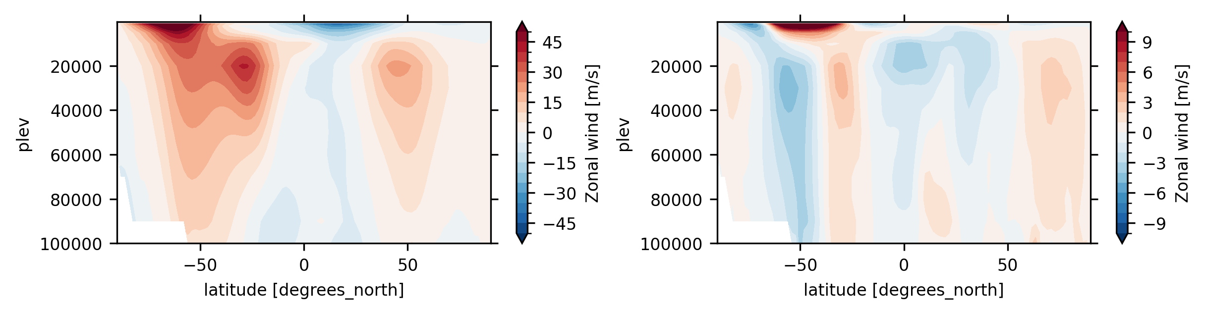
Small group discussion#
Which hemisphere has a stronger jet stream? Why? (remember that the plots are for JJA, the NH summer)
Does the mid-Holocene orbital forcing shift the jet stream?
Ask the instructors about the atmosphere circulation!
Analysis 5: how about sea-surface temperature?#
Ocean data is in
ocn/histSST is the top level of TEMP
hist_dir = '/ocn/hist/'

files_PI_ocn = glob.glob(storage_dir + case_PI + hist_dir + '*.pop.h.0001*')
files_MH_ocn = glob.glob(storage_dir + case_MH + hist_dir + '*.pop.h.0001*')
print(*files_PI_ocn, sep='\n')
print(*files_MH_ocn, sep='\n')

ds_PI_ocn = xr.open_mfdataset(
    files_PI_ocn,
    combine="by_coords",
    data_vars="minimal",
    coords="minimal",
    compat="override",
)

ds_MH_ocn = xr.open_mfdataset(
    files_MH_ocn,
    combine="by_coords",
    data_vars="minimal",
    coords="minimal",
    compat="override",
)

# Again, we need this fix to get the correct time, i.e., month 1 to month 12
ds_PI_ocn['time'] = ds_PI_ocn.time.get_index('time') - timedelta(days=15)
ds_MH_ocn['time'] = ds_MH_ocn.time.get_index('time') - timedelta(days=15)
ds_PI_ocn
Calculate annual mean SST and make a simple plot using Xarray#
sst_PI = ds_PI_ocn.TEMP.isel(z_t=0).mean('time')

sst_MH = ds_MH_ocn.TEMP.isel(z_t=0).mean('time')

sst_PI.plot(size=1.5)
What do nlat and nlon mean?
Where is Greenland? It is the “north pole” in the model!
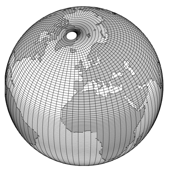
Figure: POP ocean grid
Regridding is needed!#
Use the
RegridderfromxesmfUse the
util.grid_globalto create a 1x1 regular gridUse linear interpolation
Use IPython magic command to
timethe runtime
%%time

ds_PI_ocn['lat'] = ds_PI_ocn.TLAT
ds_PI_ocn['lon'] = ds_PI_ocn.TLONG

regridder = xesmf.Regridder(
    ds_in=ds_PI_ocn,
    ds_out=xesmf.util.grid_global(1, 1, cf=True, lon1=360),
    method='bilinear',
    periodic=True)

sst_PI_1x1 = regridder(sst_PI)

sst_MH_1x1 = regridder(sst_MH)

sst_PI_1x1
lat = sst_PI_1x1.lat
lon = sst_PI_1x1.lon

fig, axes = plt.subplots(nrows=1, ncols=3,
                         figsize=(10, 2),
                         subplot_kw={'projection': ccrs.Robinson(central_longitude=210)},
                         constrained_layout=True)

ax = axes[0]
ax.set_title("PI SST, annual mean")
sst_PI_new, lon_new = add_cyclic_point(sst_PI_1x1, lon)
p0 = ax.contourf(lon_new, lat, sst_PI_new,
                 levels=np.linspace(-2, 30, 17),
                 cmap='inferno', extend='both',
                 transform=ccrs.PlateCarree())
plt.colorbar(p0, ax=ax)

ax = axes[1]
ax.set_title("MH SST, annual mean")
sst_MH_new, lon_new = add_cyclic_point(sst_MH_1x1, lon)
p1 = ax.contourf(lon_new, lat, sst_MH_new,
                 levels=np.linspace(-2, 30, 17),
                 cmap='inferno', extend='both',
                 transform=ccrs.PlateCarree())
plt.colorbar(p1, ax=ax)

ax = axes[2]
ax.set_title("MH-PI SST")
p2 = ax.contourf(lon_new, lat, sst_MH_new - sst_PI_new,
                 cmap='coolwarm',
                 levels=np.linspace(-2, 2, 21),
                 extend='both',
                 transform=ccrs.PlateCarree())
plt.colorbar(p2, ax=ax)

for ax in axes:
    ax.set_global()
    ax.coastlines(linewidth=0.5)

# We could use savefig to save the plot as pdf
# plt.savefig('SST_xy.PI_vs_MH.pdf', format='pdf', bbox_inches="tight")
Small group discussion#
Colder SSTs over lots of the regions?
What’s the timescale of upper ocean response?
We need to consider internal variability and test significance. See
4b_opt2_analyze_long_midHolocene.
Summary so far#
Load CESM output from multiple files with
XarrayPlot variables as zonal means and in map view
Interpolate the atmospheric vertical coordinate from hybrid to pressure when you need pressure levels
Ocean models use an irregular grid with the poles displaced onto land, so regridding is needed
Mid-Holocene orbital forcing is seasonal and regional, and it affects atmospheric circulation, precipitation, and other climate states