
8. Bonus: Climate Sensitivity and Feedbacks#
Tutorials at the 2026 paleoCAMP | June 15–June 29, 2026
Jiang Zhu
jiangzhu@ucar.edu
Climate & Global Dynamics Laboratory
NSF National Center for Atmospheric Research
Learning Objectives#
Understand equilibrium climate sensitivity (ECS) and effective radiative forcing (ERF)
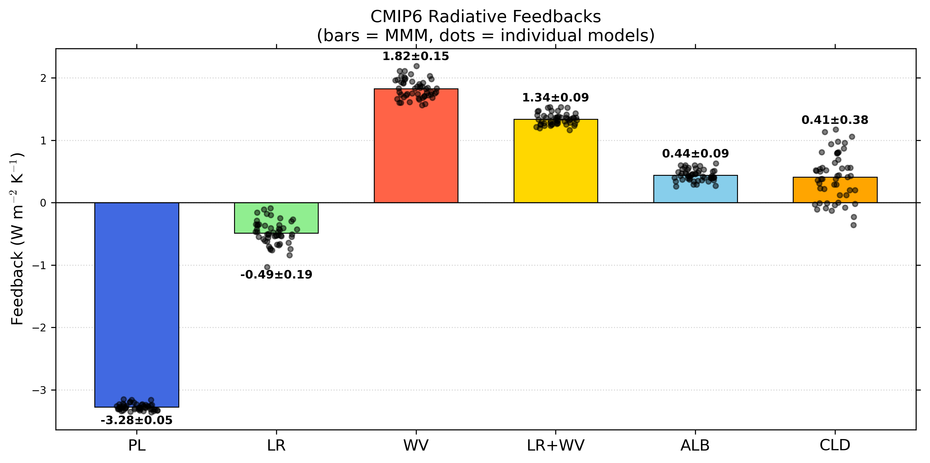
Compare ECS and the individual radiative feedbacks (Planck, lapse-rate, water-vapor, albedo, and cloud) across CMIP6 models
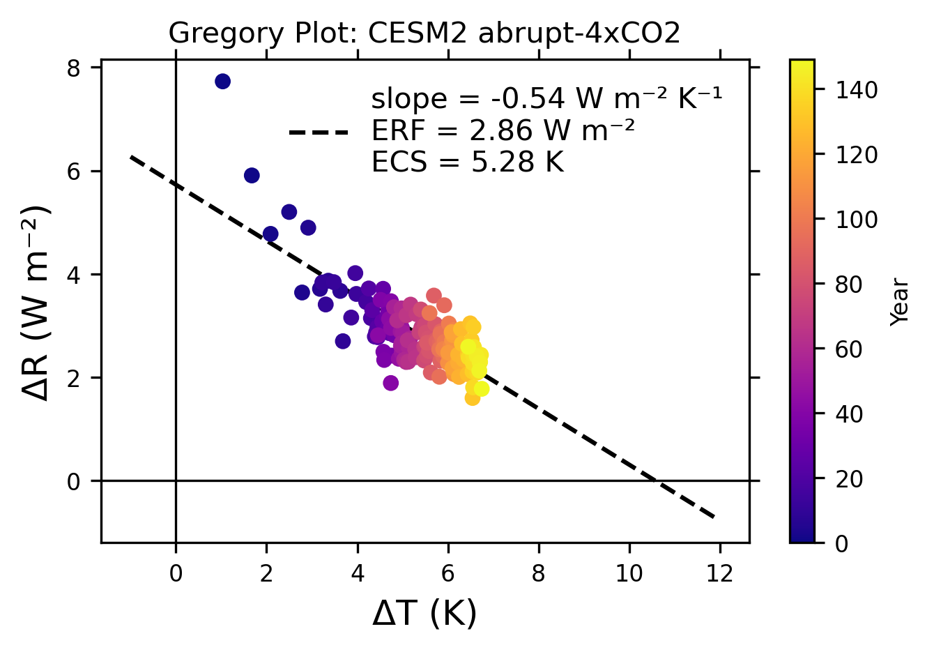
Estimate ECS and ERF from a CESM2 abrupt-4xCO2 simulation using the Gregory method
Time to learn: 15 minutes
Load Python packages
from datetime import timedelta

import xarray as xr
import numpy as np
import pandas as pd

import matplotlib.pyplot as plt

import warnings
warnings.filterwarnings("ignore")
Example 1: Look at Climate sensitivity and feedbacks in CMIP6 models with pre-computed values from Mark Zelinka#
https://github.com/mzelinka/cmip56_forcing_feedback_ecs
Zelinka, M. D., Myers, T. A., McCoy, D. T., Po-Chedley, S., Caldwell, P. M., Ceppi, P., et al. (2020). Causes of higher climate sensitivity in CMIP6 models. Geophysical Research Letters, 47, e2019GL085782. https://doi.org/10.1029/2019GL085782
url = "https://raw.githubusercontent.com/mzelinka/cmip56_forcing_feedback_ecs/master/CMIP6_ECS_ERF_fbks.txt"

df = pd.read_csv(
    url, sep=r'\s+', skiprows=10, skipfooter=4, engine='python',
    names=["Model", "Variant", "ECS", "ERF2x", "PL", "PL*", "LR",
           "LR*", "WV", "RH", "ALB", "CLD", "SWCLD",
           "LWCLD", "NET", "ERR"]
)

df = df[~df['Model'].str.startswith('-')].reset_index(drop=True)
df = df.drop(columns=["PL*", "LR*"])

df
| Model | Variant | ECS | ERF2x | PL | LR | WV | RH | ALB | CLD | SWCLD | LWCLD | NET | ERR | |
|---|---|---|---|---|---|---|---|---|---|---|---|---|---|---|
| 0 | ACCESS-ESM1-5 | r1i1p1f1 | 3.88 | 2.83 | -3.27 | -0.30 | 1.70 | 0.02 | 0.46 | 0.56 | 0.43 | 0.13 | -0.73 | 0.12 |
| 1 | AWI-CM-1-1-MR | r1i1p1f1 | 3.16 | 3.63 | -3.23 | -0.41 | 1.77 | 0.03 | 0.46 | 0.22 | -0.31 | 0.53 | -1.15 | 0.04 |
| 2 | BCC-CSM2-MR | r1i1p1f1 | 3.02 | 3.11 | -3.31 | -0.36 | 1.67 | -0.07 | 0.43 | 0.51 | 0.16 | 0.35 | -1.03 | 0.04 |
| 3 | BCC-ESM1 | r1i1p1f1 | 3.25 | 3.01 | -3.29 | -0.35 | 1.66 | -0.05 | 0.47 | 0.52 | 0.02 | 0.50 | -0.92 | 0.07 |
| 4 | CAMS-CSM1-0 | r1i1p1f1 | 2.29 | 4.17 | -3.31 | -0.62 | 2.01 | 0.05 | 0.26 | -0.36 | -0.72 | 0.36 | -1.82 | 0.19 |
| 5 | CESM2 | r1i1p1f1 | 5.15 | 3.27 | -3.34 | -0.53 | 1.87 | 0.00 | 0.40 | 0.96 | 0.79 | 0.17 | -0.63 | 0.01 |
| 6 | CESM2-FV2 | r1i1p1f1 | 5.16 | 2.86 | -3.30 | -0.51 | 1.74 | -0.07 | 0.43 | 1.06 | 0.95 | 0.11 | -0.55 | 0.03 |
| 7 | CESM2-WACCM | r1i1p1f1 | 4.68 | 3.30 | -3.34 | -0.54 | 1.86 | -0.01 | 0.40 | 1.17 | 1.05 | 0.12 | -0.71 | -0.25 |
| 8 | CESM2-WACCM-FV2 | r1i1p1f1 | 4.80 | 2.92 | -3.31 | -0.52 | 1.75 | -0.09 | 0.41 | 1.13 | 0.97 | 0.15 | -0.61 | -0.06 |
| 9 | CIESM | r1i1p1f1 | 5.63 | 3.86 | -3.25 | -0.35 | 1.60 | -0.10 | 0.29 | 0.81 | 0.68 | 0.13 | -0.69 | 0.21 |
| 10 | CMCC-CM2-SR5 | r1i1p1f1 | 3.55 | 3.79 | -3.32 | -0.47 | 1.82 | -0.01 | 0.34 | 0.52 | 0.48 | 0.04 | -1.07 | 0.04 |
| 11 | CMCC-ESM2 | r1i1p1f1 | 3.58 | 3.75 | -3.31 | -0.47 | 1.84 | 0.02 | 0.37 | 0.50 | 0.45 | 0.05 | -1.05 | 0.03 |
| 12 | CNRM-CM6-1 | r1i1p1f2 | 4.90 | 3.64 | -3.29 | -0.42 | 1.75 | -0.02 | 0.53 | 0.55 | -0.02 | 0.57 | -0.74 | 0.13 |
| 13 | CNRM-CM6-1-HR | r1i1p1f2 | 4.33 | 3.96 | -3.33 | -0.56 | 1.92 | 0.02 | 0.40 | 0.54 | -0.10 | 0.64 | -0.92 | 0.12 |
| 14 | CNRM-ESM2-1 | r1i1p1f2 | 4.79 | 2.97 | -3.29 | -0.47 | 1.83 | 0.01 | 0.51 | 0.56 | 0.03 | 0.53 | -0.62 | 0.24 |
| 15 | CanESM5 | r1i1p1f1 | 5.64 | 3.68 | -3.33 | -0.61 | 1.97 | 0.07 | 0.47 | 0.80 | -0.02 | 0.82 | -0.65 | 0.03 |
| 16 | E3SM-1-0 | r1i1p1f1 | 5.31 | 3.33 | -3.33 | -0.54 | 1.86 | 0.01 | 0.34 | 0.94 | 0.75 | 0.18 | -0.63 | 0.11 |
| 17 | EC-Earth3 | r8i1p1f1 | 4.26 | 3.22 | -3.24 | -0.16 | 1.68 | 0.11 | 0.60 | 0.31 | 0.05 | 0.26 | -0.76 | 0.05 |
| 18 | EC-Earth3-AerChem | r1i1p1f1 | 3.87 | 3.63 | -3.24 | -0.27 | 1.74 | 0.08 | 0.59 | 0.20 | -0.09 | 0.28 | -0.94 | 0.06 |
| 19 | EC-Earth3-CC | r1i1p1f1 | 4.23 | 3.25 | -3.23 | -0.25 | 1.72 | 0.09 | 0.63 | 0.29 | 0.06 | 0.23 | -0.77 | 0.07 |
| 20 | EC-Earth3-Veg | r1i1p1f1 | 4.33 | 3.37 | -3.26 | -0.20 | 1.73 | 0.11 | 0.60 | 0.29 | 0.02 | 0.27 | -0.78 | 0.07 |
| 21 | EC-Earth3-Veg-LR | r1i1p1f1 | 4.23 | 3.25 | -3.26 | -0.29 | 1.72 | 0.05 | 0.56 | 0.41 | 0.12 | 0.28 | -0.77 | 0.09 |
| 22 | FGOALS-f3-L | r1i1p1f1 | 2.98 | 4.17 | -3.20 | -0.37 | 1.65 | -0.05 | 0.40 | -0.01 | -0.21 | 0.20 | -1.40 | 0.14 |
| 23 | FGOALS-g3 | r1i1p1f1 | 2.87 | 3.58 | -3.29 | -0.37 | 1.90 | 0.14 | 0.57 | -0.01 | -0.73 | 0.72 | -1.25 | -0.06 |
| 24 | GFDL-CM4 | r1i1p1f1 | 3.89 | 3.19 | -3.24 | -0.53 | 1.84 | 0.03 | 0.55 | 0.56 | 0.03 | 0.53 | -0.82 | -0.00 |
| 25 | GFDL-ESM4 | r1i1p1f1 | 2.65 | 3.77 | -3.31 | -0.68 | 1.94 | -0.01 | 0.37 | 0.44 | -0.15 | 0.59 | -1.42 | -0.19 |
| 26 | GISS-E2-1-G | r1i1p1f1 | 2.71 | 3.95 | -3.26 | -1.03 | 2.19 | -0.01 | 0.27 | 0.00 | -0.63 | 0.64 | -1.46 | 0.37 |
| 27 | GISS-E2-1-H | r1i1p1f1 | 3.12 | 3.53 | -3.22 | -0.55 | 1.91 | 0.07 | 0.48 | -0.03 | -0.53 | 0.50 | -1.13 | 0.27 |
| 28 | GISS-E2-2-G | r1i1p1f1 | 2.43 | 3.65 | -3.24 | -0.84 | 2.11 | 0.03 | 0.39 | -0.09 | -0.88 | 0.79 | -1.51 | 0.17 |
| 29 | GISS-E2-2-H | r1i1p1f1 | 2.68 | 3.42 | -3.19 | -0.43 | 1.73 | 0.00 | 0.46 | -0.04 | -0.62 | 0.58 | -1.28 | 0.20 |
| 30 | HadGEM3-GC31-LL | r1i1p1f3 | 5.55 | 3.49 | -3.27 | -0.41 | 1.68 | -0.07 | 0.41 | 0.79 | 0.98 | -0.19 | -0.63 | 0.18 |
| 31 | HadGEM3-GC31-MM | r1i1p1f3 | 5.44 | 3.57 | -3.29 | -0.44 | 1.69 | -0.08 | 0.35 | 0.87 | 1.03 | -0.17 | -0.66 | 0.17 |
| 32 | IITM-ESM | r1i1p1f1 | 2.37 | 4.51 | -3.28 | -0.74 | 1.99 | 0.02 | 0.29 | -0.08 | -0.69 | 0.62 | -1.91 | -0.09 |
| 33 | INM-CM4-8 | r1i1p1f1 | 1.83 | 2.70 | -3.29 | -0.09 | 1.61 | 0.08 | 0.40 | -0.13 | -0.19 | 0.06 | -1.48 | 0.02 |
| 34 | INM-CM5-0 | r1i1p1f1 | 1.92 | 2.92 | -3.29 | -0.11 | 1.58 | 0.03 | 0.45 | -0.11 | -0.11 | -0.00 | -1.52 | -0.03 |
| 35 | IPSL-CM5A2-INCA | r1i1p1f1 | 3.82 | 3.07 | -3.31 | -0.73 | 2.06 | 0.04 | 0.36 | 0.98 | 0.50 | 0.48 | -0.81 | -0.17 |
| 36 | IPSL-CM6A-LR | r1i1p1f1 | 4.70 | 3.58 | -3.28 | -0.50 | 1.96 | 0.10 | 0.48 | 0.38 | 0.14 | 0.23 | -0.76 | 0.21 |
| 37 | IPSL-CM6A-LR-INCA | r1i1p1f1 | 4.13 | 3.15 | -3.28 | -0.52 | 1.93 | 0.07 | 0.49 | 0.43 | 0.19 | 0.24 | -0.76 | 0.19 |
| 38 | KACE-1-0-G | r1i1p1f1 | 4.75 | 3.41 | -3.30 | -0.51 | 1.76 | -0.07 | 0.36 | 0.80 | 0.98 | -0.19 | -0.72 | 0.18 |
| 39 | MIROC-ES2L | r1i1p1f2 | 2.66 | 4.11 | -3.31 | -0.70 | 1.98 | -0.01 | 0.44 | -0.02 | -0.35 | 0.33 | -1.54 | 0.07 |
| 40 | MIROC6 | r1i1p1f1 | 2.60 | 3.65 | -3.34 | -0.64 | 2.03 | 0.05 | 0.51 | 0.12 | -0.13 | 0.26 | -1.40 | -0.10 |
| 41 | MPI-ESM-1-2-HAM | r1i1p1f1 | 2.95 | 4.16 | -3.16 | -0.66 | 1.92 | 0.04 | 0.39 | -0.23 | -0.62 | 0.39 | -1.41 | 0.33 |
| 42 | MPI-ESM1-2-HR | r1i1p1f1 | 2.98 | 3.65 | -3.20 | -0.53 | 1.83 | 0.03 | 0.42 | 0.20 | -0.41 | 0.61 | -1.22 | 0.06 |
| 43 | MPI-ESM1-2-LR | r1i1p1f1 | 3.03 | 4.22 | -3.16 | -0.76 | 1.97 | 0.02 | 0.39 | 0.12 | -0.68 | 0.79 | -1.39 | 0.05 |
| 44 | MRI-ESM2-0 | r1i1p1f1 | 3.13 | 3.43 | -3.27 | -0.48 | 1.71 | -0.08 | 0.60 | 0.38 | 0.12 | 0.26 | -1.10 | -0.04 |
| 45 | NESM3 | r1i1p1f1 | 4.76 | 3.73 | -3.15 | -0.55 | 1.83 | 0.02 | 0.54 | 0.38 | -0.15 | 0.53 | -0.78 | 0.17 |
| 46 | NorCPM1 | r1i1p1f1 | 3.03 | 3.34 | -3.23 | -0.18 | 1.56 | -0.00 | 0.50 | 0.23 | -0.01 | 0.24 | -1.10 | 0.01 |
| 47 | NorESM2-LM | r1i1p1f1 | 2.56 | 3.43 | -3.35 | -0.67 | 2.03 | 0.03 | 0.40 | 0.36 | 0.21 | 0.15 | -1.34 | -0.10 |
| 48 | NorESM2-MM | r1i1p1f1 | 2.49 | 3.73 | -3.36 | -0.75 | 2.11 | 0.06 | 0.34 | 0.43 | 0.30 | 0.14 | -1.50 | -0.27 |
| 49 | SAM0-UNICON | r1i1p1f1 | 3.72 | 3.89 | -3.33 | -0.58 | 1.77 | -0.13 | 0.42 | 0.69 | 0.89 | -0.20 | -1.04 | -0.01 |
| 50 | TaiESM1 | r1i1p1f1 | 4.36 | 3.85 | -3.31 | -0.43 | 1.77 | -0.02 | 0.43 | 0.64 | 0.55 | 0.09 | -0.88 | 0.02 |
| 51 | UKESM1-0-LL | r1i1p1f2 | 5.36 | 3.61 | -3.26 | -0.35 | 1.60 | -0.10 | 0.53 | 0.81 | 0.93 | -0.12 | -0.67 | -0.00 |
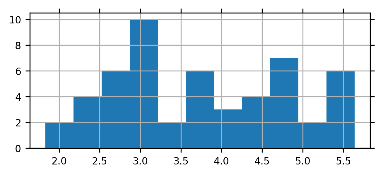
Quick plot of ECS in CMIP6 models#
df['ECS'].hist(bins=11, figsize=(5, 2))
<Axes: >
Plot of feedback strengths in CMIP6 models#
df["LR+WV"] = df["LR"] + df["WV"]

fbk_cols = ["PL", "LR", "WV", "LR+WV", "ALB", "CLD"]
fbk_colors = ["royalblue", "lightgreen", "tomato", "gold", "skyblue", "orange"]

fig, ax = plt.subplots(figsize=(10, 5))
x = np.arange(len(fbk_cols))

# MMM bars
mmm = [df[c].mean() for c in fbk_cols]
ax.bar(x, mmm, color=fbk_colors, edgecolor="k", linewidth=0.7, zorder=2, width=0.6)

# Label mean values
for i, (col, val) in enumerate(zip(fbk_cols, mmm)):
    std = df[col].std()
    if val >= 0:
        ypos = df[col].max() + 0.05
        ax.text(i, ypos, f"{val:.2f}±{std:.2f}", ha="center", va="bottom", fontsize=9, fontweight="bold")
    else:
        ypos = df[col].min() - 0.05
        ax.text(i, ypos, f"{val:.2f}±{std:.2f}", ha="center", va="top", fontsize=9, fontweight="bold")

# Individual model dots
for i, col in enumerate(fbk_cols):
    xjitter = np.random.uniform(-0.15, 0.15, len(df))
    ax.scatter(i + xjitter, df[col], color="k", s=15, alpha=0.5, zorder=3)

ax.axhline(0, color="k", linewidth=0.8)
ax.set_xticks(x)
ax.set_xticklabels(fbk_cols, fontsize=12)
ax.set_ylabel("Feedback (W m$^{-2}$ K$^{-1}$)", fontsize=12)
ax.set_title("CMIP6 Radiative Feedbacks\n(bars = MMM, dots = individual models)", fontsize=13)
ax.grid(axis="y", linestyle=":", alpha=0.5)

plt.tight_layout()
plt.show()
Example 2: Use Gregory method to plot ECS and effective radiative forcing#
def load_ds(case, suffixes):
    files = [f"{archive}/{case}/atm/proc/tseries/month_1/{case}.cam.h0.{v}.{s}"
             for v in vnames for s in suffixes]

    ds = xr.open_mfdataset(
        files,
        combine='by_coords',
        data_vars='minimal',
        coords='minimal',
        compat='override',
        parallel=True
    )
    ds['time'] = ds.time.get_index('time') - timedelta(days=15)

    return ds.resample(time='YS').mean().compute()
archive = '/glade/campaign/collections/cmip/CMIP6/timeseries-cmip6'
vnames  = ['TS', 'FSNT', 'FLNT']

case1   = 'b.e21.B1850.f19_g17.CMIP6-piControl-2deg.001'
case2   = 'b.e21.BCO2x4.f19_g17.CMIP6-abrupt4xCO2-2deg.001'
suffix1 = ['030101-035012.nc', '035101-040012.nc', '040101-045012.nc']
suffix2 = ['000101-005012.nc', '005101-010012.nc', '010101-015012.nc']

ds_ctrl = load_ds(case1, suffix1)
ds_4co2 = load_ds(case2, suffix2)
Compute temperature and net radiation anomaly in 4xCO2#
coslat = np.cos(np.deg2rad(ds_ctrl.lat))
T_ctrl = ds_ctrl.TS.weighted(coslat).mean(['lat', 'lon'])
T_4co2 = ds_4co2.TS.weighted(coslat).mean(['lat', 'lon'])
dT = T_4co2 - T_ctrl.mean('time').values

dT
<xarray.DataArray 'TS' (time: 150)> Size: 1kB
array([1.03349878, 1.67459846, 2.08804738, 2.49838632, 2.78364074,
       2.91909449, 3.17852581, 3.36114036, 3.62546262, 3.68398585,
       3.30463294, 3.23021788, 3.4829985 , 3.98096628, 3.86679891,
       3.95720756, 4.19792741, 4.38891277, 4.30227069, 4.48672866,
       4.41791873, 4.25474577, 4.44661407, 4.45274296, 4.33149851,
       4.65544854, 4.70619563, 4.57022217, 4.62761003, 4.55212042,
       4.76481635, 4.6567593 , 4.67659013, 4.81552872, 4.68729749,
       4.75641277, 4.57779737, 4.59466638, 4.51506552, 4.74403074,
       4.83839165, 4.74159298, 4.45746716, 4.70206309, 4.74501267,
       4.87721412, 4.91831655, 4.91005471, 4.98363396, 4.98193116,
       4.95716073, 4.99772022, 5.00338905, 4.96386816, 4.9753261 ,
       4.81102475, 5.16766736, 5.13925202, 5.03474146, 4.97620635,
       5.07963758, 4.88148654, 5.11351988, 5.1258168 , 5.27904357,
       5.28898994, 5.08615035, 5.17704778, 5.41501009, 5.30721871,
       5.47757247, 5.47590833, 5.37279574, 5.50230584, 5.4980305 ,
       5.49212664, 5.47521807, 5.40392305, 5.53588706, 5.51408385,
       5.57181964, 5.58316343, 5.58781514, 5.72111189, 5.54071688,
       5.71981082, 5.62338286, 5.6907707 , 5.83299878, 5.74912464,
       5.84554743, 5.82335955, 5.91982396, 5.89781759, 5.88171494,
       5.81156048, 5.83589288, 5.80690705, 5.59421694, 6.00342723,
       5.92430206, 6.02184636, 6.10539059, 5.97338404, 5.89784926,
       6.12364703, 6.14238503, 6.05818974, 6.1404125 , 6.00232942,
       6.14092503, 6.09375078, 6.13284138, 6.12822991, 6.00739327,
       6.21308301, 6.10858097, 6.09962857, 6.08298871, 6.32032836,
       6.2719881 , 6.22425499, 6.33075714, 6.24545801, 6.22712899,
       6.34166416, 6.44059539, 6.28859538, 6.4356427 , 6.30865503,
       6.49296087, 6.54425451, 6.44063564, 6.52338841, 6.56316732,
       6.543107  , 6.60183213, 6.64754602, 6.5566638 , 6.455464  ,
       6.5477804 , 6.54857521, 6.57364972, 6.72820723, 6.70912864,
       6.63423016, 6.70153449, 6.69282247, 6.44948423, 6.74685698])
Coordinates:
  * time     (time) object 1kB 0001-01-01 00:00:00 ... 0150-01-01 00:00:00
Attributes:
    units:         K
    long_name:     Surface temperature (radiative)
cell_methods: time: meanR_ctrl = (ds_ctrl.FSNT - ds_ctrl.FLNT).weighted(coslat).mean(['lat', 'lon'])
R_4co2 = (ds_4co2.FSNT - ds_4co2.FLNT).weighted(coslat).mean(['lat', 'lon'])
dR = R_4co2 - R_ctrl.mean('time').values
dR
<xarray.DataArray (time: 150)> Size: 1kB
array([7.72755333, 5.905775  , 4.77390541, 5.19888042, 3.63885816,
       4.89376233, 3.71018709, 3.86674246, 3.66966186, 2.6954044 ,
       3.40692081, 3.83253343, 3.83913546, 3.61106979, 3.15372489,
       4.0136404 , 3.45438932, 2.78582777, 3.14285688, 3.09801116,
       2.87048989, 3.7163339 , 2.96396764, 2.77381412, 3.29814053,
       3.47248533, 2.85258175, 3.71020856, 2.39018733, 3.07828731,
       2.91988124, 3.18120832, 2.95242816, 2.81174653, 3.29787275,
       2.41685915, 2.49036277, 2.33303068, 3.49590201, 3.46958831,
       3.26730565, 1.88558175, 2.81003102, 3.12546122, 2.95341161,
       3.23613596, 2.35603457, 3.15530253, 2.95864192, 2.47132717,
       2.88384384, 2.64662038, 2.8638328 , 2.60579685, 2.65614588,
       3.35311364, 2.74916939, 2.56755111, 2.33522856, 3.33081993,
       2.29375853, 3.09986051, 2.71277258, 2.29830049, 2.53736332,
       2.38696542, 3.20057893, 3.40375632, 2.96435081, 3.22009945,
       3.06494773, 2.58953302, 2.87099274, 2.89507754, 2.59738179,
       3.00753983, 2.3225079 , 3.30895255, 2.41029843, 2.86303417,
       2.75494951, 2.50762723, 2.50436562, 3.02571748, 2.66485298,
       2.71570752, 2.08893543, 3.57921511, 2.3175653 , 2.69117134,
       2.88578494, 2.66662103, 3.39216979, 2.40196819, 2.69709715,
       2.00756369, 2.84190418, 2.53765786, 3.24076208, 2.46974501,
       2.68295989, 3.03740958, 2.46877289, 2.47785469, 2.54325736,
       2.91085165, 2.05877764, 2.60382763, 2.57943254, 2.27505558,
       2.61110127, 2.71390524, 2.06225383, 2.09504392, 2.47418622,
       2.39322759, 2.8138051 , 2.17747758, 2.8700654 , 2.51405993,
       2.3584481 , 2.27997528, 2.53288953, 2.00487361, 2.4365238 ,
       2.34128297, 2.61152316, 2.92895147, 2.0590462 , 2.64652282,
       3.04025885, 1.59672861, 2.43826934, 2.71674149, 2.96989098,
       2.10777298, 2.35173492, 2.08804443, 1.80239556, 2.38161443,
       2.27206324, 2.4395087 , 2.58227912, 2.43112912, 2.29569564,
       2.41027174, 2.28201216, 2.1253328 , 2.5884508 , 1.77387667])
Coordinates:
  * time     (time) object 1kB 0001-01-01 00:00:00 ... 0150-01-01 00:00:00
Attributes:
    Sampling_Sequence:  rad_lwsw
    units:              W/m2
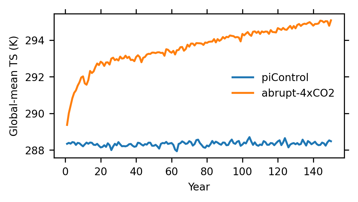
cell_methods: time: meanPlot of the warming in 4xCO2#
fig, ax = plt.subplots(figsize=(4, 2))

ax.plot(np.arange(1, len(T_ctrl) + 1), T_ctrl, label='piControl')
ax.plot(np.arange(1, len(T_4co2) + 1), T_4co2, label='abrupt-4xCO2')
ax.set_xlabel('Year')
ax.set_ylabel('Global-mean TS (K)')
ax.legend(frameon=False)
<matplotlib.legend.Legend at 0x153cc3e51400>
Linear regression and make a plot#
slope, intercept = np.polyfit(dT, dR, 1)

ECS = -intercept / slope / 2
ERF =  intercept / 2

print(f"Slope (feedback): {slope:.3f} W m⁻² K⁻¹")
print(f"ERF (2xCO2):      {ERF:.3f} W m⁻²")
print(f"ECS:              {ECS:.3f} K")
Slope (feedback): -0.542 W m⁻² K⁻¹
ERF (2xCO2):      2.863 W m⁻²
ECS:              5.281 K
# Gregory plot
fig, ax = plt.subplots(figsize=(5, 3))

years = np.arange(len(dT))
sc = ax.scatter(dT.values, dR.values, c=years, cmap='plasma', s=20, zorder=3)
plt.colorbar(sc, ax=ax, label='Year')

# Regression line
dT_line = np.linspace(-1, 12, 100)
ax.plot(dT_line, slope * dT_line + intercept, 'k--', linewidth=1.5,
        label=f"slope = {slope:.2f} W m⁻² K⁻¹\nERF = {ERF:.2f} W m⁻²\nECS = {ECS:.2f} K")

ax.axhline(0, color='k', linewidth=0.8)
ax.axvline(0, color='k', linewidth=0.8)
ax.set_xlabel('ΔT (K)', fontsize=12)
ax.set_ylabel('ΔR (W m⁻²)', fontsize=12)
ax.set_title('Gregory Plot: CESM2 abrupt-4xCO2', fontsize=10)
ax.legend(fontsize=10, frameon=False)
<matplotlib.legend.Legend at 0x153c92fdb890>