4b. Option 2: Analyze Long MidHolocene simulations

Tutorials at the 2025 paleoCAMP | June 16–June 30, 2025

Jiang Zhu
jiangzhu@ucar.edu
Climate & Global Dynamics Laboratory
NSF National Center for Atmospheric Research

---

Learning Objectives:

• Use JupyterHub to access and explore available simulation datasets

• Evaluate the role of internal climate variability by comparing plots with the one-year simulation in Section 3. Analyze CESM Output

• Understand how orbital forcing could influence the ITCZ and monsoon precipitation

• Understand how green Sahara (vegetation forcing) could influence the ITCZ and precipitation

Time to learn: 60 minutes

---

How to get started?

• Make sure you have an active JupyterHub server

• Find and open the notebook 4b_opt2_analyze_long_midHolocene in the left sidebar

• Make sure to use NPL 2025a as your Kernel (select from top right corner)

Figure: Launch a Terminal

---

Load Python packages

import os
from datetime import timedelta

import xarray as xr
import numpy as np

import matplotlib.pyplot as plt
import cartopy.crs as ccrs
from cartopy.util import add_cyclic_point

---

Analysis 1: How does orbital forcing impact the ITCZ and monsoon precipitation during the midHolocene?

• We revisit this problem using longer and better equilibrated midHolocene simulation with iCESM1.2

• Averaging over longer time (100 years here) helps to remove internal variability

The first step is to figure out the directory structure of the data

• b.e12.B1850C5.f19_g16.iPI.01 is a preindustrial control simulation of 900 model years

• b.e12.B1850C5.f19_g16.i06ka.04 is a mid-Holocene simulation of 400 years with only the orbital forcing

• Reference for the simulations: Osman et al. 2021

campaign_dir = '/glade/campaign/cgd/ppc/jiangzhu/iCESM1.2'

!ls /glade/campaign/cgd/ppc/jiangzhu/iCESM1.2

b.e12.B1850C5.f19_g16.i03ka.01
b.e12.B1850C5.f19_g16.i06ka.03
b.e12.B1850C5.f19_g16.i06ka.04
b.e12.B1850C5.f19_g16.i09ka.01
b.e12.B1850C5.f19_g16.i12ka.01
b.e12.B1850C5.f19_g16.i12ka.02
b.e12.B1850C5.f19_g16.i12ka_WH025a.01
b.e12.B1850C5.f19_g16.i14ka.01
b.e12.B1850C5.f19_g16.i16ka.01
b.e12.B1850C5.f19_g16.i16ka_WH025a.01
b.e12.B1850C5.f19_g16.i18ka.01
b.e12.B1850C5.f19_g16.i21ka.03
b.e12.B1850C5.f19_g16.i21ka.03.0kaGaI
b.e12.B1850C5.f19_g16.i21ka.03.0kaGHG
b.e12.B1850C5.f19_g16.i21ka.03.0kaICE
b.e12.B1850C5.f19_g16.iPI.01
b.e12.B1850C5.f19_g16.iPI.01.21kaGaI
b.e12.B1850C5.f19_g16.iPI.01.21kaGHG
b.e12.B1850C5.f19_g16.iPI.01.21kaICE
b.e12.B1850C5.f19_g16.iPIx2.01
extra
please_cite_tierney2020_zhu2021_osman2021

case_PI = 'b.e12.B1850C5.f19_g16.iPI.01'
case_MH = 'b.e12.B1850C5.f19_g16.i06ka.04'

# This is the folder structure under each simulation (case)
# This means atmosphere, postprocessed timeseries at monthly frequency
comp = 'atm/proc/tseries/month_1'

print('list piControl precip. files')
!ls /glade/campaign/cgd/ppc/jiangzhu/iCESM1.2/b.e12.B1850C5.f19_g16.iPI.01/atm/proc/tseries/month_1/*PRECC.*
!ls /glade/campaign/cgd/ppc/jiangzhu/iCESM1.2/b.e12.B1850C5.f19_g16.iPI.01/atm/proc/tseries/month_1/*PRECL.*

print('list midHolocene precip. files')
!ls /glade/campaign/cgd/ppc/jiangzhu/iCESM1.2/b.e12.B1850C5.f19_g16.i06ka.04/atm/proc/tseries/month_1/*PRECC.*
!ls /glade/campaign/cgd/ppc/jiangzhu/iCESM1.2/b.e12.B1850C5.f19_g16.i06ka.04/atm/proc/tseries/month_1/*PRECL.*

list piControl precip. files
/glade/campaign/cgd/ppc/jiangzhu/iCESM1.2/b.e12.B1850C5.f19_g16.iPI.01/atm/proc/tseries/month_1/b.e12.B1850C5.f19_g16.iPI.01.cam.h0.PRECC.0001-0900.cal_adj.nc
/glade/campaign/cgd/ppc/jiangzhu/iCESM1.2/b.e12.B1850C5.f19_g16.iPI.01/atm/proc/tseries/month_1/b.e12.B1850C5.f19_g16.iPI.01.cam.h0.PRECC.0001-0900.nc
/glade/campaign/cgd/ppc/jiangzhu/iCESM1.2/b.e12.B1850C5.f19_g16.iPI.01/atm/proc/tseries/month_1/b.e12.B1850C5.f19_g16.iPI.01.cam.h0.PRECL.0001-0900.cal_adj.nc
/glade/campaign/cgd/ppc/jiangzhu/iCESM1.2/b.e12.B1850C5.f19_g16.iPI.01/atm/proc/tseries/month_1/b.e12.B1850C5.f19_g16.iPI.01.cam.h0.PRECL.0001-0900.nc
list midHolocene precip. files
/glade/campaign/cgd/ppc/jiangzhu/iCESM1.2/b.e12.B1850C5.f19_g16.i06ka.04/atm/proc/tseries/month_1/b.e12.B1850C5.f19_g16.i06ka.04.cam.h0.PRECC.0001-0400.cal_adj.nc
/glade/campaign/cgd/ppc/jiangzhu/iCESM1.2/b.e12.B1850C5.f19_g16.i06ka.04/atm/proc/tseries/month_1/b.e12.B1850C5.f19_g16.i06ka.04.cam.h0.PRECC.0001-0400.nc
/glade/campaign/cgd/ppc/jiangzhu/iCESM1.2/b.e12.B1850C5.f19_g16.i06ka.04/atm/proc/tseries/month_1/b.e12.B1850C5.f19_g16.i06ka.04.cam.h0.PRECL.0001-0400.cal_adj.nc
/glade/campaign/cgd/ppc/jiangzhu/iCESM1.2/b.e12.B1850C5.f19_g16.i06ka.04/atm/proc/tseries/month_1/b.e12.B1850C5.f19_g16.i06ka.04.cam.h0.PRECL.0001-0400.nc

NOTE: files with cal_adj mean they have been corrected for the calendar effect (recall Jess’s lecture on orbital forcing)

• Create a list of files we need for piControl

# fname_precc = 'b.e12.B1850C5.f19_g16.iPI.01.cam.h0.PRECC.0001-0900.nc'
# fname_precl = 'b.e12.B1850C5.f19_g16.iPI.01.cam.h0.PRECL.0001-0900.nc'

# We use the files with calendar effect adjustments
fname_precc = 'b.e12.B1850C5.f19_g16.iPI.01.cam.h0.PRECC.0001-0900.cal_adj.nc'
fname_precl = 'b.e12.B1850C5.f19_g16.iPI.01.cam.h0.PRECL.0001-0900.cal_adj.nc'

flist_PI = [os.path.join(campaign_dir, case_PI, comp, fname_precc),
            os.path.join(campaign_dir, case_PI, comp, fname_precl)]
flist_PI

['/glade/campaign/cgd/ppc/jiangzhu/iCESM1.2/b.e12.B1850C5.f19_g16.iPI.01/atm/proc/tseries/month_1/b.e12.B1850C5.f19_g16.iPI.01.cam.h0.PRECC.0001-0900.cal_adj.nc',
 '/glade/campaign/cgd/ppc/jiangzhu/iCESM1.2/b.e12.B1850C5.f19_g16.iPI.01/atm/proc/tseries/month_1/b.e12.B1850C5.f19_g16.iPI.01.cam.h0.PRECL.0001-0900.cal_adj.nc']

• Create a list of files we need for midHolocene

# fname_precc = 'b.e12.B1850C5.f19_g16.i06ka.04.cam.h0.PRECC.0001-0400.nc'
# fname_precl = 'b.e12.B1850C5.f19_g16.i06ka.04.cam.h0.PRECL.0001-0400.nc'

# We use the files with calendar effect adjustments
fname_precc = 'b.e12.B1850C5.f19_g16.i06ka.04.cam.h0.PRECC.0001-0400.cal_adj.nc'
fname_precl = 'b.e12.B1850C5.f19_g16.i06ka.04.cam.h0.PRECL.0001-0400.cal_adj.nc'

flist_MH = [os.path.join(campaign_dir, case_MH, comp, fname_precc),
            os.path.join(campaign_dir, case_MH, comp, fname_precl)]
flist_MH

['/glade/campaign/cgd/ppc/jiangzhu/iCESM1.2/b.e12.B1850C5.f19_g16.i06ka.04/atm/proc/tseries/month_1/b.e12.B1850C5.f19_g16.i06ka.04.cam.h0.PRECC.0001-0400.cal_adj.nc',
 '/glade/campaign/cgd/ppc/jiangzhu/iCESM1.2/b.e12.B1850C5.f19_g16.i06ka.04/atm/proc/tseries/month_1/b.e12.B1850C5.f19_g16.i06ka.04.cam.h0.PRECL.0001-0400.cal_adj.nc']

Read in piControl and midHolocene data

ds_PI = xr.open_mfdataset(
    flist_PI, data_vars='minimal', coords='minimal', compat='override')

# We need this fix to get the correct time, i.e., January to December
ds_PI['time'] = ds_PI.time.get_index('time') - timedelta(days=15)

ds_PI

<xarray.Dataset> Size: 1GB
Dimensions:    (lev: 30, ilev: 31, lat: 96, lon: 144, time: 10800, nbnd: 2)
Coordinates:
  * lev        (lev) float64 240B 3.643 7.595 14.36 24.61 ... 957.5 976.3 992.6
  * ilev       (ilev) float64 248B 2.255 5.032 10.16 18.56 ... 967.5 985.1 1e+03
  * lat        (lat) float64 768B -90.0 -88.11 -86.21 ... 86.21 88.11 90.0
  * lon        (lon) float64 1kB 0.0 2.5 5.0 7.5 ... 350.0 352.5 355.0 357.5
  * time       (time) object 86kB 0001-01-16 23:08:30.912478 ... 0900-12-16 2...
Dimensions without coordinates: nbnd
Data variables: (12/25)
    hyam       (lev) float64 240B dask.array<chunksize=(30,), meta=np.ndarray>
    hybm       (lev) float64 240B dask.array<chunksize=(30,), meta=np.ndarray>
    hyai       (ilev) float64 248B dask.array<chunksize=(31,), meta=np.ndarray>
    hybi       (ilev) float64 248B dask.array<chunksize=(31,), meta=np.ndarray>
    P0         float64 8B ...
    ndbase     int32 4B ...
    ...         ...
    f11vmr     (time) float64 86kB dask.array<chunksize=(10800,), meta=np.ndarray>
    f12vmr     (time) float64 86kB dask.array<chunksize=(10800,), meta=np.ndarray>
    sol_tsi    (time) float64 86kB dask.array<chunksize=(10800,), meta=np.ndarray>
    nsteph     (time) int32 43kB dask.array<chunksize=(10800,), meta=np.ndarray>
    PRECC      (time, lat, lon) float32 597MB dask.array<chunksize=(10800, 96, 144), meta=np.ndarray>
    PRECL      (time, lat, lon) float32 597MB dask.array<chunksize=(10800, 96, 144), meta=np.ndarray>
Attributes:
    Conventions:                CF-1.0
    source:                     CAM
    case:                       b.e12.B1850C5.f19_g16.iPI.01
    title:                      UNSET
    logname:                    jiangzhu
    host:                       r5i1n15
    Version:                    $Name$
    revision_Id:                $Id$
    initial_file:               b.ie12.B1850C5CN.f19_g16.09.cam.i.0401-01-01-...
    topography_file:            /glade/p/cesmdata/cseg/inputdata/atm/cam/topo...
    paleo_calendar_adjustment:  2020-07-07 22:40:03 paleo calendar adjustment...

xarray.Dataset

• Dimensions:
  • lev: 30
  • ilev: 31
  • lat: 96
  • lon: 144
  • time: 10800
  • nbnd: 2
• Coordinates: (5)
  • lev
    (lev)
    float64
    3.643 7.595 14.36 ... 976.3 992.6

    long_name :

    hybrid level at midpoints (1000*(A+B))

    units :

    level

    positive :

    down

    standard_name :

    atmosphere_hybrid_sigma_pressure_coordinate

    formula_terms :

    a: hyam b: hybm p0: P0 ps: PS

    array([  3.643466,   7.59482 ,  14.356632,  24.61222 ,  38.2683  ,  54.59548 ,
            72.012451,  87.82123 , 103.317127, 121.547241, 142.994039, 168.22508 ,
           197.908087, 232.828619, 273.910817, 322.241902, 379.100904, 445.992574,
           524.687175, 609.778695, 691.38943 , 763.404481, 820.858369, 859.534767,
           887.020249, 912.644547, 936.198398, 957.48548 , 976.325407, 992.556095])

  • ilev
    (ilev)
    float64
    2.255 5.032 10.16 ... 985.1 1e+03

    long_name :

    hybrid level at interfaces (1000*(A+B))

    units :

    level

    positive :

    down

    standard_name :

    atmosphere_hybrid_sigma_pressure_coordinate

    formula_terms :

    a: hyai b: hybi p0: P0 ps: PS

    array([   2.25524 ,    5.031692,   10.157947,   18.555317,   30.669123,
             45.867477,   63.323483,   80.701418,   94.941042,  111.693211,
            131.401271,  154.586807,  181.863353,  213.952821,  251.704417,
            296.117216,  348.366588,  409.835219,  482.149929,  567.224421,
            652.332969,  730.445892,  796.363071,  845.353667,  873.715866,
            900.324631,  924.964462,  947.432335,  967.538625,  985.11219 ,
           1000.      ])

  • lat
    (lat)
    float64
    -90.0 -88.11 -86.21 ... 88.11 90.0

    long_name :

    latitude

    units :

    degrees_north

    array([-90.      , -88.105263, -86.210526, -84.315789, -82.421053, -80.526316,
           -78.631579, -76.736842, -74.842105, -72.947368, -71.052632, -69.157895,
           -67.263158, -65.368421, -63.473684, -61.578947, -59.684211, -57.789474,
           -55.894737, -54.      , -52.105263, -50.210526, -48.315789, -46.421053,
           -44.526316, -42.631579, -40.736842, -38.842105, -36.947368, -35.052632,
           -33.157895, -31.263158, -29.368421, -27.473684, -25.578947, -23.684211,
           -21.789474, -19.894737, -18.      , -16.105263, -14.210526, -12.315789,
           -10.421053,  -8.526316,  -6.631579,  -4.736842,  -2.842105,  -0.947368,
             0.947368,   2.842105,   4.736842,   6.631579,   8.526316,  10.421053,
            12.315789,  14.210526,  16.105263,  18.      ,  19.894737,  21.789474,
            23.684211,  25.578947,  27.473684,  29.368421,  31.263158,  33.157895,
            35.052632,  36.947368,  38.842105,  40.736842,  42.631579,  44.526316,
            46.421053,  48.315789,  50.210526,  52.105263,  54.      ,  55.894737,
            57.789474,  59.684211,  61.578947,  63.473684,  65.368421,  67.263158,
            69.157895,  71.052632,  72.947368,  74.842105,  76.736842,  78.631579,
            80.526316,  82.421053,  84.315789,  86.210526,  88.105263,  90.      ])

  • lon
    (lon)
    float64
    0.0 2.5 5.0 ... 352.5 355.0 357.5

    long_name :

    longitude

    units :

    degrees_east

    array([  0. ,   2.5,   5. ,   7.5,  10. ,  12.5,  15. ,  17.5,  20. ,  22.5,
            25. ,  27.5,  30. ,  32.5,  35. ,  37.5,  40. ,  42.5,  45. ,  47.5,
            50. ,  52.5,  55. ,  57.5,  60. ,  62.5,  65. ,  67.5,  70. ,  72.5,
            75. ,  77.5,  80. ,  82.5,  85. ,  87.5,  90. ,  92.5,  95. ,  97.5,
           100. , 102.5, 105. , 107.5, 110. , 112.5, 115. , 117.5, 120. , 122.5,
           125. , 127.5, 130. , 132.5, 135. , 137.5, 140. , 142.5, 145. , 147.5,
           150. , 152.5, 155. , 157.5, 160. , 162.5, 165. , 167.5, 170. , 172.5,
           175. , 177.5, 180. , 182.5, 185. , 187.5, 190. , 192.5, 195. , 197.5,
           200. , 202.5, 205. , 207.5, 210. , 212.5, 215. , 217.5, 220. , 222.5,
           225. , 227.5, 230. , 232.5, 235. , 237.5, 240. , 242.5, 245. , 247.5,
           250. , 252.5, 255. , 257.5, 260. , 262.5, 265. , 267.5, 270. , 272.5,
           275. , 277.5, 280. , 282.5, 285. , 287.5, 290. , 292.5, 295. , 297.5,
           300. , 302.5, 305. , 307.5, 310. , 312.5, 315. , 317.5, 320. , 322.5,
           325. , 327.5, 330. , 332.5, 335. , 337.5, 340. , 342.5, 345. , 347.5,
           350. , 352.5, 355. , 357.5])

  • time
    (time)
    object
    0001-01-16 23:08:30.912478 ... 0...

    array([cftime.DatetimeNoLeap(1, 1, 16, 23, 8, 30, 912478, has_year_zero=True),
           cftime.DatetimeNoLeap(1, 2, 13, 23, 32, 53, 395170, has_year_zero=True),
           cftime.DatetimeNoLeap(1, 3, 17, 0, 13, 21, 153924, has_year_zero=True),
           ...,
           cftime.DatetimeNoLeap(900, 10, 16, 23, 48, 9, 762855, has_year_zero=True),
           cftime.DatetimeNoLeap(900, 11, 15, 23, 16, 3, 783586, has_year_zero=True),
           cftime.DatetimeNoLeap(900, 12, 16, 23, 1, 11, 482768, has_year_zero=True)],
          dtype=object)

• Data variables: (25)
  • hyam
    (lev)
    float64
    dask.array<chunksize=(30,), meta=np.ndarray>

    long_name :

    hybrid A coefficient at layer midpoints

    Array Chunk Bytes 240 B 240 B Shape (30,) (30,) Dask graph 1 chunks in 2 graph layers Data type float64 numpy.ndarray

  • hybm
    (lev)
    float64
    dask.array<chunksize=(30,), meta=np.ndarray>

    long_name :

    hybrid B coefficient at layer midpoints

    Array Chunk Bytes 240 B 240 B Shape (30,) (30,) Dask graph 1 chunks in 2 graph layers Data type float64 numpy.ndarray

  • hyai
    (ilev)
    float64
    dask.array<chunksize=(31,), meta=np.ndarray>

    long_name :

    hybrid A coefficient at layer interfaces

    Array Chunk Bytes 248 B 248 B Shape (31,) (31,) Dask graph 1 chunks in 2 graph layers Data type float64 numpy.ndarray

  • hybi
    (ilev)
    float64
    dask.array<chunksize=(31,), meta=np.ndarray>

    long_name :

    hybrid B coefficient at layer interfaces

    Array Chunk Bytes 248 B 248 B Shape (31,) (31,) Dask graph 1 chunks in 2 graph layers Data type float64 numpy.ndarray

  • P0
    ()
    float64
    ...

    long_name :

    reference pressure

    units :

    Pa

    [1 values with dtype=float64]

  • ndbase
    ()
    int32
    ...

    long_name :

    base day

    [1 values with dtype=int32]

  • nsbase
    ()
    int32
    ...

    long_name :

    seconds of base day

    [1 values with dtype=int32]

  • nbdate
    ()
    int32
    ...

    long_name :

    base date (YYYYMMDD)

    [1 values with dtype=int32]

  • nbsec
    ()
    int32
    ...

    long_name :

    seconds of base date

    [1 values with dtype=int32]

  • mdt
    ()
    int32
    ...

    long_name :

    timestep

    units :

    s

    [1 values with dtype=int32]

  • gw
    (lat)
    float64
    dask.array<chunksize=(96,), meta=np.ndarray>

    long_name :

    gauss weights

    Array Chunk Bytes 768 B 768 B Shape (96,) (96,) Dask graph 1 chunks in 2 graph layers Data type float64 numpy.ndarray

  • date
    (time)
    int32
    dask.array<chunksize=(10800,), meta=np.ndarray>

    long_name :

    current date (YYYYMMDD)

    Array Chunk Bytes 42.19 kiB 42.19 kiB Shape (10800,) (10800,) Dask graph 1 chunks in 2 graph layers Data type int32 numpy.ndarray

  • datesec
    (time)
    int32
    dask.array<chunksize=(10800,), meta=np.ndarray>

    long_name :

    current seconds of current date

    Array Chunk Bytes 42.19 kiB 42.19 kiB Shape (10800,) (10800,) Dask graph 1 chunks in 2 graph layers Data type int32 numpy.ndarray

  • time_bnds
    (time, nbnd)
    object
    dask.array<chunksize=(10800, 2), meta=np.ndarray>

    long_name :

    time interval endpoints

    Array Chunk Bytes 168.75 kiB 168.75 kiB Shape (10800, 2) (10800, 2) Dask graph 1 chunks in 2 graph layers Data type object numpy.ndarray

  • ndcur
    (time)
    int32
    dask.array<chunksize=(10800,), meta=np.ndarray>

    long_name :

    current day (from base day)

    Array Chunk Bytes 42.19 kiB 42.19 kiB Shape (10800,) (10800,) Dask graph 1 chunks in 2 graph layers Data type int32 numpy.ndarray

  • nscur
    (time)
    int32
    dask.array<chunksize=(10800,), meta=np.ndarray>

    long_name :

    current seconds of current day

    Array Chunk Bytes 42.19 kiB 42.19 kiB Shape (10800,) (10800,) Dask graph 1 chunks in 2 graph layers Data type int32 numpy.ndarray

  • co2vmr
    (time)
    float64
    dask.array<chunksize=(10800,), meta=np.ndarray>

    long_name :

    co2 volume mixing ratio

    Array Chunk Bytes 84.38 kiB 84.38 kiB Shape (10800,) (10800,) Dask graph 1 chunks in 2 graph layers Data type float64 numpy.ndarray

  • ch4vmr
    (time)
    float64
    dask.array<chunksize=(10800,), meta=np.ndarray>

    long_name :

    ch4 volume mixing ratio

    Array Chunk Bytes 84.38 kiB 84.38 kiB Shape (10800,) (10800,) Dask graph 1 chunks in 2 graph layers Data type float64 numpy.ndarray

  • n2ovmr
    (time)
    float64
    dask.array<chunksize=(10800,), meta=np.ndarray>

    long_name :

    n2o volume mixing ratio

    Array Chunk Bytes 84.38 kiB 84.38 kiB Shape (10800,) (10800,) Dask graph 1 chunks in 2 graph layers Data type float64 numpy.ndarray

  • f11vmr
    (time)
    float64
    dask.array<chunksize=(10800,), meta=np.ndarray>

    long_name :

    f11 volume mixing ratio

    Array Chunk Bytes 84.38 kiB 84.38 kiB Shape (10800,) (10800,) Dask graph 1 chunks in 2 graph layers Data type float64 numpy.ndarray

  • f12vmr
    (time)
    float64
    dask.array<chunksize=(10800,), meta=np.ndarray>

    long_name :

    f12 volume mixing ratio

    Array Chunk Bytes 84.38 kiB 84.38 kiB Shape (10800,) (10800,) Dask graph 1 chunks in 2 graph layers Data type float64 numpy.ndarray

  • sol_tsi
    (time)
    float64
    dask.array<chunksize=(10800,), meta=np.ndarray>

    long_name :

    total solar irradiance

    units :

    W/m2

    Array Chunk Bytes 84.38 kiB 84.38 kiB Shape (10800,) (10800,) Dask graph 1 chunks in 2 graph layers Data type float64 numpy.ndarray

  • nsteph
    (time)
    int32
    dask.array<chunksize=(10800,), meta=np.ndarray>

    long_name :

    current timestep

    Array Chunk Bytes 42.19 kiB 42.19 kiB Shape (10800,) (10800,) Dask graph 1 chunks in 2 graph layers Data type int32 numpy.ndarray

  • PRECC
    (time, lat, lon)
    float32
    dask.array<chunksize=(10800, 96, 144), meta=np.ndarray>

    units :

    m/s

    long_name :

    Convective precipitation rate (liq + ice)

    cell_methods :

    time: mean

    paleo_calendar_adjustment :

    monthly values adjusted for the appropriate paleo calendar

    Array Chunk Bytes 569.53 MiB 569.53 MiB Shape (10800, 96, 144) (10800, 96, 144) Dask graph 1 chunks in 2 graph layers Data type float32 numpy.ndarray

  • PRECL
    (time, lat, lon)
    float32
    dask.array<chunksize=(10800, 96, 144), meta=np.ndarray>

    units :

    m/s

    long_name :

    Large-scale (stable) precipitation rate (liq + ice)

    cell_methods :

    time: mean

    paleo_calendar_adjustment :

    monthly values adjusted for the appropriate paleo calendar

    Array Chunk Bytes 569.53 MiB 569.53 MiB Shape (10800, 96, 144) (10800, 96, 144) Dask graph 1 chunks in 2 graph layers Data type float32 numpy.ndarray

• Indexes: (5)
  • lev
    PandasIndex

    PandasIndex(Index([  3.64346569404006,  7.594819646328688, 14.356632251292467,
           24.612220004200935,  38.26829977333546,  54.59547974169254,
            72.01245054602623,  87.82123029232025, 103.31712663173676,
           121.54724076390266, 142.99403876066208, 168.22507977485657,
            197.9080867022276, 232.82861895859241,  273.9108167588711,
            322.2419023513794, 379.10090386867523,   445.992574095726,
            524.6871747076511,  609.7786948084831,  691.3894303143024,
             763.404481112957,  820.8583686500788,  859.5347665250301,
            887.0202489197254,   912.644546944648,  936.1983984708786,
             957.485479535535,   976.325407391414,   992.556095123291],
          dtype='float64', name='lev'))

  • ilev
    PandasIndex

    PandasIndex(Index([ 2.255239523947239,  5.031691864132881,  10.15794742852449,
            18.55531707406044,  30.66912293434143,  45.86747661232948,
             63.3234828710556,  80.70141822099686,  94.94104236364365,
           111.69321089982991,  131.4012706279755,  154.5868068933487,
            181.8633526563644, 213.95282074809072, 251.70441716909409,
           296.11721634864807,  348.3665883541107,  409.8352193832398,
           482.14992880821234,    567.22442060709,  652.3329690098763,
            730.4458916187286,  796.3630706071854,  845.3536666929722,
            873.7158663570881,  900.3246314823627,  924.9644624069333,
            947.4323345348239,  967.5386245362461,   985.112190246582,
                       1000.0],
          dtype='float64', name='ilev'))

  • lat
    PandasIndex

    PandasIndex(Index([              -90.0,  -88.10526315789474,  -86.21052631578948,
             -84.3157894736842,  -82.42105263157895,  -80.52631578947368,
            -78.63157894736842,  -76.73684210526316,  -74.84210526315789,
            -72.94736842105263,  -71.05263157894737,  -69.15789473684211,
            -67.26315789473685,  -65.36842105263158, -63.473684210526315,
           -61.578947368421055, -59.684210526315795,  -57.78947368421053,
            -55.89473684210527,               -54.0,  -52.10526315789474,
            -50.21052631578947,  -48.31578947368421,  -46.42105263157895,
           -44.526315789473685, -42.631578947368425,  -40.73684210526316,
             -38.8421052631579,  -36.94736842105264,  -35.05263157894737,
            -33.15789473684211, -31.263157894736842, -29.368421052631582,
           -27.473684210526322, -25.578947368421055, -23.684210526315795,
           -21.789473684210535,  -19.89473684210526,               -18.0,
            -16.10526315789474,  -14.21052631578948,  -12.31578947368422,
           -10.421052631578945,  -8.526315789473685,  -6.631578947368425,
            -4.736842105263165, -2.8421052631579045, -0.9473684210526301,
            0.9473684210526301,  2.8421052631578902,    4.73684210526315,
             6.631578947368411,   8.526315789473685,  10.421052631578945,
            12.315789473684205,  14.210526315789465,  16.105263157894726,
                          18.0,   19.89473684210526,   21.78947368421052,
             23.68421052631578,   25.57894736842104,  27.473684210526315,
            29.368421052631575,  31.263157894736835,  33.157894736842096,
            35.052631578947356,   36.94736842105263,   38.84210526315789,
             40.73684210526315,   42.63157894736841,   44.52631578947367,
             46.42105263157893,   48.31578947368419,   50.21052631578948,
             52.10526315789474,                54.0,   55.89473684210526,
             57.78947368421052,   59.68421052631578,   61.57894736842104,
              63.4736842105263,   65.36842105263156,   67.26315789473682,
             69.15789473684211,   71.05263157894737,   72.94736842105263,
             74.84210526315789,   76.73684210526315,   78.63157894736841,
             80.52631578947367,   82.42105263157893,   84.31578947368419,
             86.21052631578945,   88.10526315789474,                90.0],
          dtype='float64', name='lat'))

  • lon
    PandasIndex

    PandasIndex(Index([  0.0,   2.5,   5.0,   7.5,  10.0,  12.5,  15.0,  17.5,  20.0,  22.5,
           ...
           335.0, 337.5, 340.0, 342.5, 345.0, 347.5, 350.0, 352.5, 355.0, 357.5],
          dtype='float64', name='lon', length=144))

  • time
    PandasIndex

    PandasIndex(CFTimeIndex([0001-01-16 23:08:30.912478, 0001-02-13 23:32:53.395170, 0001-03-17 00:13:21.153924,
                 0001-04-16 00:56:09.078125, 0001-05-17 01:31:54.225442, 0001-06-16 01:48:15.511881,
                 0001-07-17 01:41:12.862833, 0001-08-17 01:12:09.032653, 0001-09-16 00:31:25.305438,
                 0001-10-16 23:48:09.762855,
                 ...
                 0900-03-17 00:13:21.153922, 0900-04-16 00:56:09.078125, 0900-05-17 01:31:54.225442,
                 0900-06-16 01:48:15.511881, 0900-07-17 01:41:12.862831, 0900-08-17 01:12:09.032655,
                 0900-09-16 00:31:25.305440, 0900-10-16 23:48:09.762855, 0900-11-15 23:16:03.783586,
                 0900-12-16 23:01:11.482768],
                dtype='object', length=10800, calendar='noleap', freq=None))

• Attributes: (11)

  Conventions :

  CF-1.0

  source :

  CAM

  case :

  b.e12.B1850C5.f19_g16.iPI.01

  title :

  UNSET

  logname :

  jiangzhu

  host :

  r5i1n15

  Version :

  $Name$

  revision_Id :

  $Id$

  initial_file :

  b.ie12.B1850C5CN.f19_g16.09.cam.i.0401-01-01-00000.nc

  topography_file :

  /glade/p/cesmdata/cseg/inputdata/atm/cam/topo/USGS-gtopo30_1.9x2.5_remap_c050602.nc

  paleo_calendar_adjustment :

  2020-07-07 22:40:03 paleo calendar adjustment by cal_adjust_PMIP.f90

• Select the last 100 years using .sel

ds_PI = ds_PI.sel(time=slice('0801', '0900'))
ds_PI

<xarray.Dataset> Size: 133MB
Dimensions:    (lev: 30, ilev: 31, lat: 96, lon: 144, time: 1200, nbnd: 2)
Coordinates:
  * lev        (lev) float64 240B 3.643 7.595 14.36 24.61 ... 957.5 976.3 992.6
  * ilev       (ilev) float64 248B 2.255 5.032 10.16 18.56 ... 967.5 985.1 1e+03
  * lat        (lat) float64 768B -90.0 -88.11 -86.21 ... 86.21 88.11 90.0
  * lon        (lon) float64 1kB 0.0 2.5 5.0 7.5 ... 350.0 352.5 355.0 357.5
  * time       (time) object 10kB 0801-01-16 23:08:30.912476 ... 0900-12-16 2...
Dimensions without coordinates: nbnd
Data variables: (12/25)
    hyam       (lev) float64 240B dask.array<chunksize=(30,), meta=np.ndarray>
    hybm       (lev) float64 240B dask.array<chunksize=(30,), meta=np.ndarray>
    hyai       (ilev) float64 248B dask.array<chunksize=(31,), meta=np.ndarray>
    hybi       (ilev) float64 248B dask.array<chunksize=(31,), meta=np.ndarray>
    P0         float64 8B ...
    ndbase     int32 4B ...
    ...         ...
    f11vmr     (time) float64 10kB dask.array<chunksize=(1200,), meta=np.ndarray>
    f12vmr     (time) float64 10kB dask.array<chunksize=(1200,), meta=np.ndarray>
    sol_tsi    (time) float64 10kB dask.array<chunksize=(1200,), meta=np.ndarray>
    nsteph     (time) int32 5kB dask.array<chunksize=(1200,), meta=np.ndarray>
    PRECC      (time, lat, lon) float32 66MB dask.array<chunksize=(1200, 96, 144), meta=np.ndarray>
    PRECL      (time, lat, lon) float32 66MB dask.array<chunksize=(1200, 96, 144), meta=np.ndarray>
Attributes:
    Conventions:                CF-1.0
    source:                     CAM
    case:                       b.e12.B1850C5.f19_g16.iPI.01
    title:                      UNSET
    logname:                    jiangzhu
    host:                       r5i1n15
    Version:                    $Name$
    revision_Id:                $Id$
    initial_file:               b.ie12.B1850C5CN.f19_g16.09.cam.i.0401-01-01-...
    topography_file:            /glade/p/cesmdata/cseg/inputdata/atm/cam/topo...
    paleo_calendar_adjustment:  2020-07-07 22:40:03 paleo calendar adjustment...

xarray.Dataset

• Dimensions:
  • lev: 30
  • ilev: 31
  • lat: 96
  • lon: 144
  • time: 1200
  • nbnd: 2
• Coordinates: (5)
  • lev
    (lev)
    float64
    3.643 7.595 14.36 ... 976.3 992.6

    long_name :

    hybrid level at midpoints (1000*(A+B))

    units :

    level

    positive :

    down

    standard_name :

    atmosphere_hybrid_sigma_pressure_coordinate

    formula_terms :

    a: hyam b: hybm p0: P0 ps: PS

    array([  3.643466,   7.59482 ,  14.356632,  24.61222 ,  38.2683  ,  54.59548 ,
            72.012451,  87.82123 , 103.317127, 121.547241, 142.994039, 168.22508 ,
           197.908087, 232.828619, 273.910817, 322.241902, 379.100904, 445.992574,
           524.687175, 609.778695, 691.38943 , 763.404481, 820.858369, 859.534767,
           887.020249, 912.644547, 936.198398, 957.48548 , 976.325407, 992.556095])

  • ilev
    (ilev)
    float64
    2.255 5.032 10.16 ... 985.1 1e+03

    long_name :

    hybrid level at interfaces (1000*(A+B))

    units :

    level

    positive :

    down

    standard_name :

    atmosphere_hybrid_sigma_pressure_coordinate

    formula_terms :

    a: hyai b: hybi p0: P0 ps: PS

    array([   2.25524 ,    5.031692,   10.157947,   18.555317,   30.669123,
             45.867477,   63.323483,   80.701418,   94.941042,  111.693211,
            131.401271,  154.586807,  181.863353,  213.952821,  251.704417,
            296.117216,  348.366588,  409.835219,  482.149929,  567.224421,
            652.332969,  730.445892,  796.363071,  845.353667,  873.715866,
            900.324631,  924.964462,  947.432335,  967.538625,  985.11219 ,
           1000.      ])

  • lat
    (lat)
    float64
    -90.0 -88.11 -86.21 ... 88.11 90.0

    long_name :

    latitude

    units :

    degrees_north

    array([-90.      , -88.105263, -86.210526, -84.315789, -82.421053, -80.526316,
           -78.631579, -76.736842, -74.842105, -72.947368, -71.052632, -69.157895,
           -67.263158, -65.368421, -63.473684, -61.578947, -59.684211, -57.789474,
           -55.894737, -54.      , -52.105263, -50.210526, -48.315789, -46.421053,
           -44.526316, -42.631579, -40.736842, -38.842105, -36.947368, -35.052632,
           -33.157895, -31.263158, -29.368421, -27.473684, -25.578947, -23.684211,
           -21.789474, -19.894737, -18.      , -16.105263, -14.210526, -12.315789,
           -10.421053,  -8.526316,  -6.631579,  -4.736842,  -2.842105,  -0.947368,
             0.947368,   2.842105,   4.736842,   6.631579,   8.526316,  10.421053,
            12.315789,  14.210526,  16.105263,  18.      ,  19.894737,  21.789474,
            23.684211,  25.578947,  27.473684,  29.368421,  31.263158,  33.157895,
            35.052632,  36.947368,  38.842105,  40.736842,  42.631579,  44.526316,
            46.421053,  48.315789,  50.210526,  52.105263,  54.      ,  55.894737,
            57.789474,  59.684211,  61.578947,  63.473684,  65.368421,  67.263158,
            69.157895,  71.052632,  72.947368,  74.842105,  76.736842,  78.631579,
            80.526316,  82.421053,  84.315789,  86.210526,  88.105263,  90.      ])

  • lon
    (lon)
    float64
    0.0 2.5 5.0 ... 352.5 355.0 357.5

    long_name :

    longitude

    units :

    degrees_east

    array([  0. ,   2.5,   5. ,   7.5,  10. ,  12.5,  15. ,  17.5,  20. ,  22.5,
            25. ,  27.5,  30. ,  32.5,  35. ,  37.5,  40. ,  42.5,  45. ,  47.5,
            50. ,  52.5,  55. ,  57.5,  60. ,  62.5,  65. ,  67.5,  70. ,  72.5,
            75. ,  77.5,  80. ,  82.5,  85. ,  87.5,  90. ,  92.5,  95. ,  97.5,
           100. , 102.5, 105. , 107.5, 110. , 112.5, 115. , 117.5, 120. , 122.5,
           125. , 127.5, 130. , 132.5, 135. , 137.5, 140. , 142.5, 145. , 147.5,
           150. , 152.5, 155. , 157.5, 160. , 162.5, 165. , 167.5, 170. , 172.5,
           175. , 177.5, 180. , 182.5, 185. , 187.5, 190. , 192.5, 195. , 197.5,
           200. , 202.5, 205. , 207.5, 210. , 212.5, 215. , 217.5, 220. , 222.5,
           225. , 227.5, 230. , 232.5, 235. , 237.5, 240. , 242.5, 245. , 247.5,
           250. , 252.5, 255. , 257.5, 260. , 262.5, 265. , 267.5, 270. , 272.5,
           275. , 277.5, 280. , 282.5, 285. , 287.5, 290. , 292.5, 295. , 297.5,
           300. , 302.5, 305. , 307.5, 310. , 312.5, 315. , 317.5, 320. , 322.5,
           325. , 327.5, 330. , 332.5, 335. , 337.5, 340. , 342.5, 345. , 347.5,
           350. , 352.5, 355. , 357.5])

  • time
    (time)
    object
    0801-01-16 23:08:30.912476 ... 0...

    array([cftime.DatetimeNoLeap(801, 1, 16, 23, 8, 30, 912476, has_year_zero=True),
           cftime.DatetimeNoLeap(801, 2, 13, 23, 32, 53, 395169, has_year_zero=True),
           cftime.DatetimeNoLeap(801, 3, 17, 0, 13, 21, 153922, has_year_zero=True),
           ...,
           cftime.DatetimeNoLeap(900, 10, 16, 23, 48, 9, 762855, has_year_zero=True),
           cftime.DatetimeNoLeap(900, 11, 15, 23, 16, 3, 783586, has_year_zero=True),
           cftime.DatetimeNoLeap(900, 12, 16, 23, 1, 11, 482768, has_year_zero=True)],
          dtype=object)

• Data variables: (25)
  • hyam
    (lev)
    float64
    dask.array<chunksize=(30,), meta=np.ndarray>

    long_name :

    hybrid A coefficient at layer midpoints

    Array Chunk Bytes 240 B 240 B Shape (30,) (30,) Dask graph 1 chunks in 2 graph layers Data type float64 numpy.ndarray

  • hybm
    (lev)
    float64
    dask.array<chunksize=(30,), meta=np.ndarray>

    long_name :

    hybrid B coefficient at layer midpoints

    Array Chunk Bytes 240 B 240 B Shape (30,) (30,) Dask graph 1 chunks in 2 graph layers Data type float64 numpy.ndarray

  • hyai
    (ilev)
    float64
    dask.array<chunksize=(31,), meta=np.ndarray>

    long_name :

    hybrid A coefficient at layer interfaces

    Array Chunk Bytes 248 B 248 B Shape (31,) (31,) Dask graph 1 chunks in 2 graph layers Data type float64 numpy.ndarray

  • hybi
    (ilev)
    float64
    dask.array<chunksize=(31,), meta=np.ndarray>

    long_name :

    hybrid B coefficient at layer interfaces

    Array Chunk Bytes 248 B 248 B Shape (31,) (31,) Dask graph 1 chunks in 2 graph layers Data type float64 numpy.ndarray

  • P0
    ()
    float64
    ...

    long_name :

    reference pressure

    units :

    Pa

    [1 values with dtype=float64]

  • ndbase
    ()
    int32
    ...

    long_name :

    base day

    [1 values with dtype=int32]

  • nsbase
    ()
    int32
    ...

    long_name :

    seconds of base day

    [1 values with dtype=int32]

  • nbdate
    ()
    int32
    ...

    long_name :

    base date (YYYYMMDD)

    [1 values with dtype=int32]

  • nbsec
    ()
    int32
    ...

    long_name :

    seconds of base date

    [1 values with dtype=int32]

  • mdt
    ()
    int32
    ...

    long_name :

    timestep

    units :

    s

    [1 values with dtype=int32]

  • gw
    (lat)
    float64
    dask.array<chunksize=(96,), meta=np.ndarray>

    long_name :

    gauss weights

    Array Chunk Bytes 768 B 768 B Shape (96,) (96,) Dask graph 1 chunks in 2 graph layers Data type float64 numpy.ndarray

  • date
    (time)
    int32
    dask.array<chunksize=(1200,), meta=np.ndarray>

    long_name :

    current date (YYYYMMDD)

    Array Chunk Bytes 4.69 kiB 4.69 kiB Shape (1200,) (1200,) Dask graph 1 chunks in 3 graph layers Data type int32 numpy.ndarray

  • datesec
    (time)
    int32
    dask.array<chunksize=(1200,), meta=np.ndarray>

    long_name :

    current seconds of current date

    Array Chunk Bytes 4.69 kiB 4.69 kiB Shape (1200,) (1200,) Dask graph 1 chunks in 3 graph layers Data type int32 numpy.ndarray

  • time_bnds
    (time, nbnd)
    object
    dask.array<chunksize=(1200, 2), meta=np.ndarray>

    long_name :

    time interval endpoints

    Array Chunk Bytes 18.75 kiB 18.75 kiB Shape (1200, 2) (1200, 2) Dask graph 1 chunks in 3 graph layers Data type object numpy.ndarray

  • ndcur
    (time)
    int32
    dask.array<chunksize=(1200,), meta=np.ndarray>

    long_name :

    current day (from base day)

    Array Chunk Bytes 4.69 kiB 4.69 kiB Shape (1200,) (1200,) Dask graph 1 chunks in 3 graph layers Data type int32 numpy.ndarray

  • nscur
    (time)
    int32
    dask.array<chunksize=(1200,), meta=np.ndarray>

    long_name :

    current seconds of current day

    Array Chunk Bytes 4.69 kiB 4.69 kiB Shape (1200,) (1200,) Dask graph 1 chunks in 3 graph layers Data type int32 numpy.ndarray

  • co2vmr
    (time)
    float64
    dask.array<chunksize=(1200,), meta=np.ndarray>

    long_name :

    co2 volume mixing ratio

    Array Chunk Bytes 9.38 kiB 9.38 kiB Shape (1200,) (1200,) Dask graph 1 chunks in 3 graph layers Data type float64 numpy.ndarray

  • ch4vmr
    (time)
    float64
    dask.array<chunksize=(1200,), meta=np.ndarray>

    long_name :

    ch4 volume mixing ratio

    Array Chunk Bytes 9.38 kiB 9.38 kiB Shape (1200,) (1200,) Dask graph 1 chunks in 3 graph layers Data type float64 numpy.ndarray

  • n2ovmr
    (time)
    float64
    dask.array<chunksize=(1200,), meta=np.ndarray>

    long_name :

    n2o volume mixing ratio

    Array Chunk Bytes 9.38 kiB 9.38 kiB Shape (1200,) (1200,) Dask graph 1 chunks in 3 graph layers Data type float64 numpy.ndarray

  • f11vmr
    (time)
    float64
    dask.array<chunksize=(1200,), meta=np.ndarray>

    long_name :

    f11 volume mixing ratio

    Array Chunk Bytes 9.38 kiB 9.38 kiB Shape (1200,) (1200,) Dask graph 1 chunks in 3 graph layers Data type float64 numpy.ndarray

  • f12vmr
    (time)
    float64
    dask.array<chunksize=(1200,), meta=np.ndarray>

    long_name :

    f12 volume mixing ratio

    Array Chunk Bytes 9.38 kiB 9.38 kiB Shape (1200,) (1200,) Dask graph 1 chunks in 3 graph layers Data type float64 numpy.ndarray

  • sol_tsi
    (time)
    float64
    dask.array<chunksize=(1200,), meta=np.ndarray>

    long_name :

    total solar irradiance

    units :

    W/m2

    Array Chunk Bytes 9.38 kiB 9.38 kiB Shape (1200,) (1200,) Dask graph 1 chunks in 3 graph layers Data type float64 numpy.ndarray

  • nsteph
    (time)
    int32
    dask.array<chunksize=(1200,), meta=np.ndarray>

    long_name :

    current timestep

    Array Chunk Bytes 4.69 kiB 4.69 kiB Shape (1200,) (1200,) Dask graph 1 chunks in 3 graph layers Data type int32 numpy.ndarray

  • PRECC
    (time, lat, lon)
    float32
    dask.array<chunksize=(1200, 96, 144), meta=np.ndarray>

    units :

    m/s

    long_name :

    Convective precipitation rate (liq + ice)

    cell_methods :

    time: mean

    paleo_calendar_adjustment :

    monthly values adjusted for the appropriate paleo calendar

    Array Chunk Bytes 63.28 MiB 63.28 MiB Shape (1200, 96, 144) (1200, 96, 144) Dask graph 1 chunks in 3 graph layers Data type float32 numpy.ndarray

  • PRECL
    (time, lat, lon)
    float32
    dask.array<chunksize=(1200, 96, 144), meta=np.ndarray>

    units :

    m/s

    long_name :

    Large-scale (stable) precipitation rate (liq + ice)

    cell_methods :

    time: mean

    paleo_calendar_adjustment :

    monthly values adjusted for the appropriate paleo calendar

    Array Chunk Bytes 63.28 MiB 63.28 MiB Shape (1200, 96, 144) (1200, 96, 144) Dask graph 1 chunks in 3 graph layers Data type float32 numpy.ndarray

• Indexes: (5)
  • lev
    PandasIndex

    PandasIndex(Index([  3.64346569404006,  7.594819646328688, 14.356632251292467,
           24.612220004200935,  38.26829977333546,  54.59547974169254,
            72.01245054602623,  87.82123029232025, 103.31712663173676,
           121.54724076390266, 142.99403876066208, 168.22507977485657,
            197.9080867022276, 232.82861895859241,  273.9108167588711,
            322.2419023513794, 379.10090386867523,   445.992574095726,
            524.6871747076511,  609.7786948084831,  691.3894303143024,
             763.404481112957,  820.8583686500788,  859.5347665250301,
            887.0202489197254,   912.644546944648,  936.1983984708786,
             957.485479535535,   976.325407391414,   992.556095123291],
          dtype='float64', name='lev'))

  • ilev
    PandasIndex

    PandasIndex(Index([ 2.255239523947239,  5.031691864132881,  10.15794742852449,
            18.55531707406044,  30.66912293434143,  45.86747661232948,
             63.3234828710556,  80.70141822099686,  94.94104236364365,
           111.69321089982991,  131.4012706279755,  154.5868068933487,
            181.8633526563644, 213.95282074809072, 251.70441716909409,
           296.11721634864807,  348.3665883541107,  409.8352193832398,
           482.14992880821234,    567.22442060709,  652.3329690098763,
            730.4458916187286,  796.3630706071854,  845.3536666929722,
            873.7158663570881,  900.3246314823627,  924.9644624069333,
            947.4323345348239,  967.5386245362461,   985.112190246582,
                       1000.0],
          dtype='float64', name='ilev'))

  • lat
    PandasIndex

    PandasIndex(Index([              -90.0,  -88.10526315789474,  -86.21052631578948,
             -84.3157894736842,  -82.42105263157895,  -80.52631578947368,
            -78.63157894736842,  -76.73684210526316,  -74.84210526315789,
            -72.94736842105263,  -71.05263157894737,  -69.15789473684211,
            -67.26315789473685,  -65.36842105263158, -63.473684210526315,
           -61.578947368421055, -59.684210526315795,  -57.78947368421053,
            -55.89473684210527,               -54.0,  -52.10526315789474,
            -50.21052631578947,  -48.31578947368421,  -46.42105263157895,
           -44.526315789473685, -42.631578947368425,  -40.73684210526316,
             -38.8421052631579,  -36.94736842105264,  -35.05263157894737,
            -33.15789473684211, -31.263157894736842, -29.368421052631582,
           -27.473684210526322, -25.578947368421055, -23.684210526315795,
           -21.789473684210535,  -19.89473684210526,               -18.0,
            -16.10526315789474,  -14.21052631578948,  -12.31578947368422,
           -10.421052631578945,  -8.526315789473685,  -6.631578947368425,
            -4.736842105263165, -2.8421052631579045, -0.9473684210526301,
            0.9473684210526301,  2.8421052631578902,    4.73684210526315,
             6.631578947368411,   8.526315789473685,  10.421052631578945,
            12.315789473684205,  14.210526315789465,  16.105263157894726,
                          18.0,   19.89473684210526,   21.78947368421052,
             23.68421052631578,   25.57894736842104,  27.473684210526315,
            29.368421052631575,  31.263157894736835,  33.157894736842096,
            35.052631578947356,   36.94736842105263,   38.84210526315789,
             40.73684210526315,   42.63157894736841,   44.52631578947367,
             46.42105263157893,   48.31578947368419,   50.21052631578948,
             52.10526315789474,                54.0,   55.89473684210526,
             57.78947368421052,   59.68421052631578,   61.57894736842104,
              63.4736842105263,   65.36842105263156,   67.26315789473682,
             69.15789473684211,   71.05263157894737,   72.94736842105263,
             74.84210526315789,   76.73684210526315,   78.63157894736841,
             80.52631578947367,   82.42105263157893,   84.31578947368419,
             86.21052631578945,   88.10526315789474,                90.0],
          dtype='float64', name='lat'))

  • lon
    PandasIndex

    PandasIndex(Index([  0.0,   2.5,   5.0,   7.5,  10.0,  12.5,  15.0,  17.5,  20.0,  22.5,
           ...
           335.0, 337.5, 340.0, 342.5, 345.0, 347.5, 350.0, 352.5, 355.0, 357.5],
          dtype='float64', name='lon', length=144))

  • time
    PandasIndex

    PandasIndex(CFTimeIndex([0801-01-16 23:08:30.912476, 0801-02-13 23:32:53.395169, 0801-03-17 00:13:21.153922,
                 0801-04-16 00:56:09.078125, 0801-05-17 01:31:54.225442, 0801-06-16 01:48:15.511881,
                 0801-07-17 01:41:12.862831, 0801-08-17 01:12:09.032655, 0801-09-16 00:31:25.305440,
                 0801-10-16 23:48:09.762855,
                 ...
                 0900-03-17 00:13:21.153922, 0900-04-16 00:56:09.078125, 0900-05-17 01:31:54.225442,
                 0900-06-16 01:48:15.511881, 0900-07-17 01:41:12.862831, 0900-08-17 01:12:09.032655,
                 0900-09-16 00:31:25.305440, 0900-10-16 23:48:09.762855, 0900-11-15 23:16:03.783586,
                 0900-12-16 23:01:11.482768],
                dtype='object', length=1200, calendar='noleap', freq=None))

• Attributes: (11)

  Conventions :

  CF-1.0

  source :

  CAM

  case :

  b.e12.B1850C5.f19_g16.iPI.01

  title :

  UNSET

  logname :

  jiangzhu

  host :

  r5i1n15

  Version :

  $Name$

  revision_Id :

  $Id$

  initial_file :

  b.ie12.B1850C5CN.f19_g16.09.cam.i.0401-01-01-00000.nc

  topography_file :

  /glade/p/cesmdata/cseg/inputdata/atm/cam/topo/USGS-gtopo30_1.9x2.5_remap_c050602.nc

  paleo_calendar_adjustment :

  2020-07-07 22:40:03 paleo calendar adjustment by cal_adjust_PMIP.f90

• Repeat for midHolocene

ds_MH = xr.open_mfdataset(
    flist_MH, data_vars='minimal', coords='minimal', compat='override')

# We need this fix to get the correct time, i.e., January to December
ds_MH['time'] = ds_MH.time.get_index('time') - timedelta(days=15)
ds_MH = ds_MH.sel(time=slice('0301', '0400'))

ds_MH

<xarray.Dataset> Size: 133MB
Dimensions:    (lev: 30, ilev: 31, lat: 96, lon: 144, time: 1200, nbnd: 2)
Coordinates:
  * lev        (lev) float64 240B 3.643 7.595 14.36 24.61 ... 957.5 976.3 992.6
  * ilev       (ilev) float64 248B 2.255 5.032 10.16 18.56 ... 967.5 985.1 1e+03
  * lat        (lat) float64 768B -90.0 -88.11 -86.21 ... 86.21 88.11 90.0
  * lon        (lon) float64 1kB 0.0 2.5 5.0 7.5 ... 350.0 352.5 355.0 357.5
  * time       (time) object 10kB 0301-01-14 09:41:24.727502 ... 0400-12-12 2...
Dimensions without coordinates: nbnd
Data variables: (12/25)
    hyam       (lev) float64 240B dask.array<chunksize=(30,), meta=np.ndarray>
    hybm       (lev) float64 240B dask.array<chunksize=(30,), meta=np.ndarray>
    hyai       (ilev) float64 248B dask.array<chunksize=(31,), meta=np.ndarray>
    hybi       (ilev) float64 248B dask.array<chunksize=(31,), meta=np.ndarray>
    P0         float64 8B ...
    ndbase     int32 4B ...
    ...         ...
    f11vmr     (time) float64 10kB dask.array<chunksize=(1200,), meta=np.ndarray>
    f12vmr     (time) float64 10kB dask.array<chunksize=(1200,), meta=np.ndarray>
    sol_tsi    (time) float64 10kB dask.array<chunksize=(1200,), meta=np.ndarray>
    nsteph     (time) int32 5kB dask.array<chunksize=(1200,), meta=np.ndarray>
    PRECC      (time, lat, lon) float32 66MB dask.array<chunksize=(1200, 96, 144), meta=np.ndarray>
    PRECL      (time, lat, lon) float32 66MB dask.array<chunksize=(1200, 96, 144), meta=np.ndarray>
Attributes:
    Conventions:                CF-1.0
    source:                     CAM
    case:                       b.e12.B1850C5.f19_g16.i06ka.04
    title:                      UNSET
    logname:                    jiangzhu
    host:                       r2i0n29
    Version:                    $Name$
    revision_Id:                $Id$
    initial_file:               b.e12.B1850C5.f19_g16.i06ka.03.cam.i.0901-01-...
    topography_file:            /glade/work/jiangzhu/data/inputdata/cesm120ka...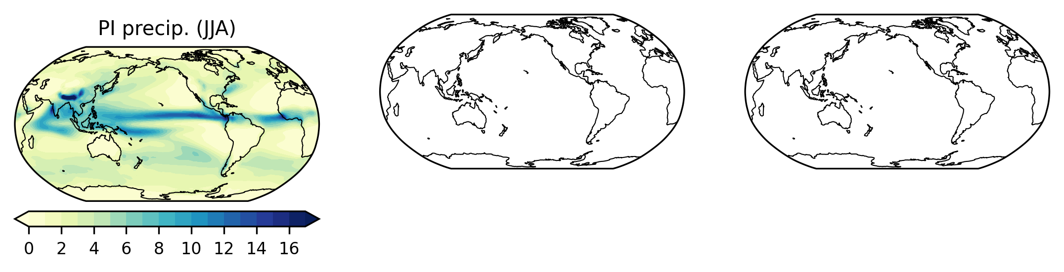
    paleo_calendar_adjustment:  2020-09-29 01:04:27 paleo calendar adjustment...

xarray.Dataset

• Dimensions:
  • lev: 30
  • ilev: 31
  • lat: 96
  • lon: 144
  • time: 1200
  • nbnd: 2
• Coordinates: (5)
  • lev
    (lev)
    float64
    3.643 7.595 14.36 ... 976.3 992.6

    long_name :

    hybrid level at midpoints (1000*(A+B))

    units :

    level

    positive :

    down

    standard_name :

    atmosphere_hybrid_sigma_pressure_coordinate

    formula_terms :

    a: hyam b: hybm p0: P0 ps: PS

    array([  3.643466,   7.59482 ,  14.356632,  24.61222 ,  38.2683  ,  54.59548 ,
            72.012451,  87.82123 , 103.317127, 121.547241, 142.994039, 168.22508 ,
           197.908087, 232.828619, 273.910817, 322.241902, 379.100904, 445.992574,
           524.687175, 609.778695, 691.38943 , 763.404481, 820.858369, 859.534767,
           887.020249, 912.644547, 936.198398, 957.48548 , 976.325407, 992.556095])

  • ilev
    (ilev)
    float64
    2.255 5.032 10.16 ... 985.1 1e+03

    long_name :

    hybrid level at interfaces (1000*(A+B))

    units :

    level

    positive :

    down

    standard_name :

    atmosphere_hybrid_sigma_pressure_coordinate

    formula_terms :

    a: hyai b: hybi p0: P0 ps: PS

    array([   2.25524 ,    5.031692,   10.157947,   18.555317,   30.669123,
             45.867477,   63.323483,   80.701418,   94.941042,  111.693211,
            131.401271,  154.586807,  181.863353,  213.952821,  251.704417,
            296.117216,  348.366588,  409.835219,  482.149929,  567.224421,
            652.332969,  730.445892,  796.363071,  845.353667,  873.715866,
            900.324631,  924.964462,  947.432335,  967.538625,  985.11219 ,
           1000.      ])

  • lat
    (lat)
    float64
    -90.0 -88.11 -86.21 ... 88.11 90.0

    long_name :

    latitude

    units :

    degrees_north

    array([-90.      , -88.105263, -86.210526, -84.315789, -82.421053, -80.526316,
           -78.631579, -76.736842, -74.842105, -72.947368, -71.052632, -69.157895,
           -67.263158, -65.368421, -63.473684, -61.578947, -59.684211, -57.789474,
           -55.894737, -54.      , -52.105263, -50.210526, -48.315789, -46.421053,
           -44.526316, -42.631579, -40.736842, -38.842105, -36.947368, -35.052632,
           -33.157895, -31.263158, -29.368421, -27.473684, -25.578947, -23.684211,
           -21.789474, -19.894737, -18.      , -16.105263, -14.210526, -12.315789,
           -10.421053,  -8.526316,  -6.631579,  -4.736842,  -2.842105,  -0.947368,
             0.947368,   2.842105,   4.736842,   6.631579,   8.526316,  10.421053,
            12.315789,  14.210526,  16.105263,  18.      ,  19.894737,  21.789474,
            23.684211,  25.578947,  27.473684,  29.368421,  31.263158,  33.157895,
            35.052632,  36.947368,  38.842105,  40.736842,  42.631579,  44.526316,
            46.421053,  48.315789,  50.210526,  52.105263,  54.      ,  55.894737,
            57.789474,  59.684211,  61.578947,  63.473684,  65.368421,  67.263158,
            69.157895,  71.052632,  72.947368,  74.842105,  76.736842,  78.631579,
            80.526316,  82.421053,  84.315789,  86.210526,  88.105263,  90.      ])

  • lon
    (lon)
    float64
    0.0 2.5 5.0 ... 352.5 355.0 357.5

    long_name :

    longitude

    units :

    degrees_east

    array([  0. ,   2.5,   5. ,   7.5,  10. ,  12.5,  15. ,  17.5,  20. ,  22.5,
            25. ,  27.5,  30. ,  32.5,  35. ,  37.5,  40. ,  42.5,  45. ,  47.5,
            50. ,  52.5,  55. ,  57.5,  60. ,  62.5,  65. ,  67.5,  70. ,  72.5,
            75. ,  77.5,  80. ,  82.5,  85. ,  87.5,  90. ,  92.5,  95. ,  97.5,
           100. , 102.5, 105. , 107.5, 110. , 112.5, 115. , 117.5, 120. , 122.5,
           125. , 127.5, 130. , 132.5, 135. , 137.5, 140. , 142.5, 145. , 147.5,
           150. , 152.5, 155. , 157.5, 160. , 162.5, 165. , 167.5, 170. , 172.5,
           175. , 177.5, 180. , 182.5, 185. , 187.5, 190. , 192.5, 195. , 197.5,
           200. , 202.5, 205. , 207.5, 210. , 212.5, 215. , 217.5, 220. , 222.5,
           225. , 227.5, 230. , 232.5, 235. , 237.5, 240. , 242.5, 245. , 247.5,
           250. , 252.5, 255. , 257.5, 260. , 262.5, 265. , 267.5, 270. , 272.5,
           275. , 277.5, 280. , 282.5, 285. , 287.5, 290. , 292.5, 295. , 297.5,
           300. , 302.5, 305. , 307.5, 310. , 312.5, 315. , 317.5, 320. , 322.5,
           325. , 327.5, 330. , 332.5, 335. , 337.5, 340. , 342.5, 345. , 347.5,
           350. , 352.5, 355. , 357.5])

  • time
    (time)
    object
    0301-01-14 09:41:24.727502 ... 0...

    array([cftime.DatetimeNoLeap(301, 1, 14, 9, 41, 24, 727502, has_year_zero=True),
           cftime.DatetimeNoLeap(301, 2, 12, 22, 12, 51, 509325, has_year_zero=True),
           cftime.DatetimeNoLeap(301, 3, 17, 9, 40, 35, 684539, has_year_zero=True),
           ...,
           cftime.DatetimeNoLeap(400, 10, 12, 1, 42, 44, 850790, has_year_zero=True),
           cftime.DatetimeNoLeap(400, 11, 11, 2, 25, 1, 843291, has_year_zero=True),
           cftime.DatetimeNoLeap(400, 12, 12, 22, 41, 59, 257646, has_year_zero=True)],
          dtype=object)

• Data variables: (25)
  • hyam
    (lev)
    float64
    dask.array<chunksize=(30,), meta=np.ndarray>

    long_name :

    hybrid A coefficient at layer midpoints

    Array Chunk Bytes 240 B 240 B Shape (30,) (30,) Dask graph 1 chunks in 2 graph layers Data type float64 numpy.ndarray

  • hybm
    (lev)
    float64
    dask.array<chunksize=(30,), meta=np.ndarray>

    long_name :

    hybrid B coefficient at layer midpoints

    Array Chunk Bytes 240 B 240 B Shape (30,) (30,) Dask graph 1 chunks in 2 graph layers Data type float64 numpy.ndarray

  • hyai
    (ilev)
    float64
    dask.array<chunksize=(31,), meta=np.ndarray>

    long_name :

    hybrid A coefficient at layer interfaces

    Array Chunk Bytes 248 B 248 B Shape (31,) (31,) Dask graph 1 chunks in 2 graph layers Data type float64 numpy.ndarray

  • hybi
    (ilev)
    float64
    dask.array<chunksize=(31,), meta=np.ndarray>

    long_name :

    hybrid B coefficient at layer interfaces

    Array Chunk Bytes 248 B 248 B Shape (31,) (31,) Dask graph 1 chunks in 2 graph layers Data type float64 numpy.ndarray

  • P0
    ()
    float64
    ...

    long_name :

    reference pressure

    units :

    Pa

    [1 values with dtype=float64]

  • ndbase
    ()
    int32
    ...

    long_name :

    base day

    [1 values with dtype=int32]

  • nsbase
    ()
    int32
    ...

    long_name :

    seconds of base day

    [1 values with dtype=int32]

  • nbdate
    ()
    int32
    ...

    long_name :

    base date (YYYYMMDD)

    [1 values with dtype=int32]

  • nbsec
    ()
    int32
    ...

    long_name :

    seconds of base date

    [1 values with dtype=int32]

  • mdt
    ()
    int32
    ...

    long_name :

    timestep

    units :

    s

    [1 values with dtype=int32]

  • gw
    (lat)
    float64
    dask.array<chunksize=(96,), meta=np.ndarray>

    long_name :

    gauss weights

    Array Chunk Bytes 768 B 768 B Shape (96,) (96,) Dask graph 1 chunks in 2 graph layers Data type float64 numpy.ndarray

  • date
    (time)
    int32
    dask.array<chunksize=(1200,), meta=np.ndarray>

    long_name :

    current date (YYYYMMDD)

    Array Chunk Bytes 4.69 kiB 4.69 kiB Shape (1200,) (1200,) Dask graph 1 chunks in 3 graph layers Data type int32 numpy.ndarray

  • datesec
    (time)
    int32
    dask.array<chunksize=(1200,), meta=np.ndarray>

    long_name :

    current seconds of current date

    Array Chunk Bytes 4.69 kiB 4.69 kiB Shape (1200,) (1200,) Dask graph 1 chunks in 3 graph layers Data type int32 numpy.ndarray

  • time_bnds
    (time, nbnd)
    object
    dask.array<chunksize=(1200, 2), meta=np.ndarray>

    long_name :

    time interval endpoints

    Array Chunk Bytes 18.75 kiB 18.75 kiB Shape (1200, 2) (1200, 2) Dask graph 1 chunks in 3 graph layers Data type object numpy.ndarray

  • ndcur
    (time)
    int32
    dask.array<chunksize=(1200,), meta=np.ndarray>

    long_name :

    current day (from base day)

    Array Chunk Bytes 4.69 kiB 4.69 kiB Shape (1200,) (1200,) Dask graph 1 chunks in 3 graph layers Data type int32 numpy.ndarray

  • nscur
    (time)
    int32
    dask.array<chunksize=(1200,), meta=np.ndarray>

    long_name :

    current seconds of current day

    Array Chunk Bytes 4.69 kiB 4.69 kiB Shape (1200,) (1200,) Dask graph 1 chunks in 3 graph layers Data type int32 numpy.ndarray

  • co2vmr
    (time)
    float64
    dask.array<chunksize=(1200,), meta=np.ndarray>

    long_name :

    co2 volume mixing ratio

    Array Chunk Bytes 9.38 kiB 9.38 kiB Shape (1200,) (1200,) Dask graph 1 chunks in 3 graph layers Data type float64 numpy.ndarray

  • ch4vmr
    (time)
    float64
    dask.array<chunksize=(1200,), meta=np.ndarray>

    long_name :

    ch4 volume mixing ratio

    Array Chunk Bytes 9.38 kiB 9.38 kiB Shape (1200,) (1200,) Dask graph 1 chunks in 3 graph layers Data type float64 numpy.ndarray

  • n2ovmr
    (time)
    float64
    dask.array<chunksize=(1200,), meta=np.ndarray>

    long_name :

    n2o volume mixing ratio

    Array Chunk Bytes 9.38 kiB 9.38 kiB Shape (1200,) (1200,) Dask graph 1 chunks in 3 graph layers Data type float64 numpy.ndarray

  • f11vmr
    (time)
    float64
    dask.array<chunksize=(1200,), meta=np.ndarray>

    long_name :

    f11 volume mixing ratio

    Array Chunk Bytes 9.38 kiB 9.38 kiB Shape (1200,) (1200,) Dask graph 1 chunks in 3 graph layers Data type float64 numpy.ndarray

  • f12vmr
    (time)
    float64
    dask.array<chunksize=(1200,), meta=np.ndarray>

    long_name :

    f12 volume mixing ratio

    Array Chunk Bytes 9.38 kiB 9.38 kiB Shape (1200,) (1200,) Dask graph 1 chunks in 3 graph layers Data type float64 numpy.ndarray

  • sol_tsi
    (time)
    float64
    dask.array<chunksize=(1200,), meta=np.ndarray>

    long_name :

    total solar irradiance

    units :

    W/m2

    Array Chunk Bytes 9.38 kiB 9.38 kiB Shape (1200,) (1200,) Dask graph 1 chunks in 3 graph layers Data type float64 numpy.ndarray

  • nsteph
    (time)
    int32
    dask.array<chunksize=(1200,), meta=np.ndarray>

    long_name :

    current timestep

    Array Chunk Bytes 4.69 kiB 4.69 kiB Shape (1200,) (1200,) Dask graph 1 chunks in 3 graph layers Data type int32 numpy.ndarray

  • PRECC
    (time, lat, lon)
    float32
    dask.array<chunksize=(1200, 96, 144), meta=np.ndarray>

    units :

    m/s

    long_name :

    Convective precipitation rate (liq + ice)

    cell_methods :

    time: mean

    paleo_calendar_adjustment :

    monthly values adjusted for the appropriate paleo calendar

    Array Chunk Bytes 63.28 MiB 63.28 MiB Shape (1200, 96, 144) (1200, 96, 144) Dask graph 1 chunks in 3 graph layers Data type float32 numpy.ndarray

  • PRECL
    (time, lat, lon)
    float32
    dask.array<chunksize=(1200, 96, 144), meta=np.ndarray>

    units :

    m/s

    long_name :

    Large-scale (stable) precipitation rate (liq + ice)

    cell_methods :

    time: mean

    paleo_calendar_adjustment :

    monthly values adjusted for the appropriate paleo calendar

    Array Chunk Bytes 63.28 MiB 63.28 MiB Shape (1200, 96, 144) (1200, 96, 144) Dask graph 1 chunks in 3 graph layers Data type float32 numpy.ndarray

• Indexes: (5)
  • lev
    PandasIndex

    PandasIndex(Index([  3.64346569404006,  7.594819646328688, 14.356632251292467,
           24.612220004200935,  38.26829977333546,  54.59547974169254,
            72.01245054602623,  87.82123029232025, 103.31712663173676,
           121.54724076390266, 142.99403876066208, 168.22507977485657,
            197.9080867022276, 232.82861895859241,  273.9108167588711,
            322.2419023513794, 379.10090386867523,   445.992574095726,
            524.6871747076511,  609.7786948084831,  691.3894303143024,
             763.404481112957,  820.8583686500788,  859.5347665250301,
            887.0202489197254,   912.644546944648,  936.1983984708786,
             957.485479535535,   976.325407391414,   992.556095123291],
          dtype='float64', name='lev'))

  • ilev
    PandasIndex

    PandasIndex(Index([ 2.255239523947239,  5.031691864132881,  10.15794742852449,
            18.55531707406044,  30.66912293434143,  45.86747661232948,
             63.3234828710556,  80.70141822099686,  94.94104236364365,
           111.69321089982991,  131.4012706279755,  154.5868068933487,
            181.8633526563644, 213.95282074809072, 251.70441716909409,
           296.11721634864807,  348.3665883541107,  409.8352193832398,
           482.14992880821234,    567.22442060709,  652.3329690098763,
            730.4458916187286,  796.3630706071854,  845.3536666929722,
            873.7158663570881,  900.3246314823627,  924.9644624069333,
            947.4323345348239,  967.5386245362461,   985.112190246582,
                       1000.0],
          dtype='float64', name='ilev'))

  • lat
    PandasIndex

    PandasIndex(Index([              -90.0,  -88.10526315789474,  -86.21052631578948,
             -84.3157894736842,  -82.42105263157895,  -80.52631578947368,
            -78.63157894736842,  -76.73684210526316,  -74.84210526315789,
            -72.94736842105263,  -71.05263157894737,  -69.15789473684211,
            -67.26315789473685,  -65.36842105263158, -63.473684210526315,
           -61.578947368421055, -59.684210526315795,  -57.78947368421053,
            -55.89473684210527,               -54.0,  -52.10526315789474,
            -50.21052631578947,  -48.31578947368421,  -46.42105263157895,
           -44.526315789473685, -42.631578947368425,  -40.73684210526316,
             -38.8421052631579,  -36.94736842105264,  -35.05263157894737,
            -33.15789473684211, -31.263157894736842, -29.368421052631582,
           -27.473684210526322, -25.578947368421055, -23.684210526315795,
           -21.789473684210535,  -19.89473684210526,               -18.0,
            -16.10526315789474,  -14.21052631578948,  -12.31578947368422,
           -10.421052631578945,  -8.526315789473685,  -6.631578947368425,
            -4.736842105263165, -2.8421052631579045, -0.9473684210526301,
            0.9473684210526301,  2.8421052631578902,    4.73684210526315,
             6.631578947368411,   8.526315789473685,  10.421052631578945,
            12.315789473684205,  14.210526315789465,  16.105263157894726,
                          18.0,   19.89473684210526,   21.78947368421052,
             23.68421052631578,   25.57894736842104,  27.473684210526315,
            29.368421052631575,  31.263157894736835,  33.157894736842096,
            35.052631578947356,   36.94736842105263,   38.84210526315789,
             40.73684210526315,   42.63157894736841,   44.52631578947367,
             46.42105263157893,   48.31578947368419,   50.21052631578948,
             52.10526315789474,                54.0,   55.89473684210526,
             57.78947368421052,   59.68421052631578,   61.57894736842104,
              63.4736842105263,   65.36842105263156,   67.26315789473682,
             69.15789473684211,   71.05263157894737,   72.94736842105263,
             74.84210526315789,   76.73684210526315,   78.63157894736841,
             80.52631578947367,   82.42105263157893,   84.31578947368419,
             86.21052631578945,   88.10526315789474,                90.0],
          dtype='float64', name='lat'))

  • lon
    PandasIndex

    PandasIndex(Index([  0.0,   2.5,   5.0,   7.5,  10.0,  12.5,  15.0,  17.5,  20.0,  22.5,
           ...
           335.0, 337.5, 340.0, 342.5, 345.0, 347.5, 350.0, 352.5, 355.0, 357.5],
          dtype='float64', name='lon', length=144))

  • time
    PandasIndex

    PandasIndex(CFTimeIndex([0301-01-14 09:41:24.727502, 0301-02-12 22:12:51.509325, 0301-03-17 09:40:35.684539,
                 0301-04-17 05:37:24.704772, 0301-05-18 05:24:37.044454, 0301-06-16 09:09:50.691910,
                 0301-07-15 21:39:03.357480, 0301-08-14 05:29:32.970651, 0301-09-11 20:39:52.311527,
                 0301-10-12 01:42:44.850790,
                 ...
                 0400-03-17 09:40:35.684541, 0400-04-17 05:37:24.704771, 0400-05-18 05:24:37.044454,
                 0400-06-16 09:09:50.691910, 0400-07-15 21:39:03.357479, 0400-08-14 05:29:32.970650,
                 0400-09-11 20:39:52.311527, 0400-10-12 01:42:44.850790, 0400-11-11 02:25:01.843291,
                 0400-12-12 22:41:59.257646],
                dtype='object', length=1200, calendar='noleap', freq=None))

• Attributes: (11)

  Conventions :

  CF-1.0

  source :

  CAM

  case :

  b.e12.B1850C5.f19_g16.i06ka.04

  title :

  UNSET

  logname :

  jiangzhu

  host :

  r2i0n29

  Version :

  $Name$

  revision_Id :

  $Id$

  initial_file :

  b.e12.B1850C5.f19_g16.i06ka.03.cam.i.0901-01-01-00000.nc

  topography_file :

  /glade/work/jiangzhu/data/inputdata/cesm120ka_ICEG6/6ka/topo_6ka_remap_19x25.mod.171206.sm9.nc

  paleo_calendar_adjustment :

  2020-09-29 01:04:27 paleo calendar adjustment by cal_adjust_PMIP.f90

Compute the NH summer mean (JJA)

m_p_s_to_mm_p_day = 86400000

• piControl

# Recall Kevin's method to compute JJA mean
ds_PI_JJA = ds_PI.groupby('time.season').mean(dim='time').sel(season='JJA')

prec_PI = (ds_PI_JJA.PRECC + ds_PI_JJA.PRECL) * m_p_s_to_mm_p_day

prec_PI

<xarray.DataArray (lat: 96, lon: 144)> Size: 111kB
dask.array<mul, shape=(96, 144), dtype=float64, chunksize=(96, 144), chunktype=numpy.ndarray>
Coordinates:
  * lat      (lat) float64 768B -90.0 -88.11 -86.21 -84.32 ... 86.21 88.11 90.0
  * lon      (lon) float64 1kB 0.0 2.5 5.0 7.5 10.0 ... 350.0 352.5 355.0 357.5
    season   <U3 12B 'JJA'

xarray.DataArray

• lat: 96
• lon: 144

• dask.array<chunksize=(96, 144), meta=np.ndarray>

  Array Chunk Bytes 108.00 kiB 108.00 kiB Shape (96, 144) (96, 144) Dask graph 1 chunks in 19 graph layers Data type float64 numpy.ndarray

• Coordinates: (3)
  • lat
    (lat)
    float64
    -90.0 -88.11 -86.21 ... 88.11 90.0

    long_name :

    latitude

    units :

    degrees_north

    array([-90.      , -88.105263, -86.210526, -84.315789, -82.421053, -80.526316,
           -78.631579, -76.736842, -74.842105, -72.947368, -71.052632, -69.157895,
           -67.263158, -65.368421, -63.473684, -61.578947, -59.684211, -57.789474,
           -55.894737, -54.      , -52.105263, -50.210526, -48.315789, -46.421053,
           -44.526316, -42.631579, -40.736842, -38.842105, -36.947368, -35.052632,
           -33.157895, -31.263158, -29.368421, -27.473684, -25.578947, -23.684211,
           -21.789474, -19.894737, -18.      , -16.105263, -14.210526, -12.315789,
           -10.421053,  -8.526316,  -6.631579,  -4.736842,  -2.842105,  -0.947368,
             0.947368,   2.842105,   4.736842,   6.631579,   8.526316,  10.421053,
            12.315789,  14.210526,  16.105263,  18.      ,  19.894737,  21.789474,
            23.684211,  25.578947,  27.473684,  29.368421,  31.263158,  33.157895,
            35.052632,  36.947368,  38.842105,  40.736842,  42.631579,  44.526316,
            46.421053,  48.315789,  50.210526,  52.105263,  54.      ,  55.894737,
            57.789474,  59.684211,  61.578947,  63.473684,  65.368421,  67.263158,
            69.157895,  71.052632,  72.947368,  74.842105,  76.736842,  78.631579,
            80.526316,  82.421053,  84.315789,  86.210526,  88.105263,  90.      ])

  • lon
    (lon)
    float64
    0.0 2.5 5.0 ... 352.5 355.0 357.5

    long_name :

    longitude

    units :

    degrees_east

    array([  0. ,   2.5,   5. ,   7.5,  10. ,  12.5,  15. ,  17.5,  20. ,  22.5,
            25. ,  27.5,  30. ,  32.5,  35. ,  37.5,  40. ,  42.5,  45. ,  47.5,
            50. ,  52.5,  55. ,  57.5,  60. ,  62.5,  65. ,  67.5,  70. ,  72.5,
            75. ,  77.5,  80. ,  82.5,  85. ,  87.5,  90. ,  92.5,  95. ,  97.5,
           100. , 102.5, 105. , 107.5, 110. , 112.5, 115. , 117.5, 120. , 122.5,
           125. , 127.5, 130. , 132.5, 135. , 137.5, 140. , 142.5, 145. , 147.5,
           150. , 152.5, 155. , 157.5, 160. , 162.5, 165. , 167.5, 170. , 172.5,
           175. , 177.5, 180. , 182.5, 185. , 187.5, 190. , 192.5, 195. , 197.5,
           200. , 202.5, 205. , 207.5, 210. , 212.5, 215. , 217.5, 220. , 222.5,
           225. , 227.5, 230. , 232.5, 235. , 237.5, 240. , 242.5, 245. , 247.5,
           250. , 252.5, 255. , 257.5, 260. , 262.5, 265. , 267.5, 270. , 272.5,
           275. , 277.5, 280. , 282.5, 285. , 287.5, 290. , 292.5, 295. , 297.5,
           300. , 302.5, 305. , 307.5, 310. , 312.5, 315. , 317.5, 320. , 322.5,
           325. , 327.5, 330. , 332.5, 335. , 337.5, 340. , 342.5, 345. , 347.5,
           350. , 352.5, 355. , 357.5])

  • season
    ()
    <U3
    'JJA'

    array('JJA', dtype='<U3')

• Indexes: (2)
  • lat
    PandasIndex

    PandasIndex(Index([              -90.0,  -88.10526315789474,  -86.21052631578948,
             -84.3157894736842,  -82.42105263157895,  -80.52631578947368,
            -78.63157894736842,  -76.73684210526316,  -74.84210526315789,
            -72.94736842105263,  -71.05263157894737,  -69.15789473684211,
            -67.26315789473685,  -65.36842105263158, -63.473684210526315,
           -61.578947368421055, -59.684210526315795,  -57.78947368421053,
            -55.89473684210527,               -54.0,  -52.10526315789474,
            -50.21052631578947,  -48.31578947368421,  -46.42105263157895,
           -44.526315789473685, -42.631578947368425,  -40.73684210526316,
             -38.8421052631579,  -36.94736842105264,  -35.05263157894737,
            -33.15789473684211, -31.263157894736842, -29.368421052631582,
           -27.473684210526322, -25.578947368421055, -23.684210526315795,
           -21.789473684210535,  -19.89473684210526,               -18.0,
            -16.10526315789474,  -14.21052631578948,  -12.31578947368422,
           -10.421052631578945,  -8.526315789473685,  -6.631578947368425,
            -4.736842105263165, -2.8421052631579045, -0.9473684210526301,
            0.9473684210526301,  2.8421052631578902,    4.73684210526315,
             6.631578947368411,   8.526315789473685,  10.421052631578945,
            12.315789473684205,  14.210526315789465,  16.105263157894726,
                          18.0,   19.89473684210526,   21.78947368421052,
             23.68421052631578,   25.57894736842104,  27.473684210526315,
            29.368421052631575,  31.263157894736835,  33.157894736842096,
            35.052631578947356,   36.94736842105263,   38.84210526315789,
             40.73684210526315,   42.63157894736841,   44.52631578947367,
             46.42105263157893,   48.31578947368419,   50.21052631578948,
             52.10526315789474,                54.0,   55.89473684210526,
             57.78947368421052,   59.68421052631578,   61.57894736842104,
              63.4736842105263,   65.36842105263156,   67.26315789473682,
             69.15789473684211,   71.05263157894737,   72.94736842105263,
             74.84210526315789,   76.73684210526315,   78.63157894736841,
             80.52631578947367,   82.42105263157893,   84.31578947368419,
             86.21052631578945,   88.10526315789474,                90.0],
          dtype='float64', name='lat'))

  • lon
    PandasIndex

    PandasIndex(Index([  0.0,   2.5,   5.0,   7.5,  10.0,  12.5,  15.0,  17.5,  20.0,  22.5,
           ...
           335.0, 337.5, 340.0, 342.5, 345.0, 347.5, 350.0, 352.5, 355.0, 357.5],
          dtype='float64', name='lon', length=144))

• Attributes: (0)

• Task 1: Add your code for midHolocene using ds_MH

Click here for the solution

Copy and paste the code into the above cell

ds_MH_JJA = ds_MH.groupby('time.season').mean(dim='time').sel(season='JJA')

prec_MH = (ds_MH_JJA.PRECC + ds_MH_JJA.PRECL) * m_p_s_to_mm_p_day

prec_MH

Plot JJA precipitation for piControl, midHolocene, and the difference between them

• I have an example on how to plot the JJA mean precipitation from piControl

• Task 2: Add your own code below to plot that for midHolocene

• Task 3: Add your own code below to plot the anomaly (midHolocene - piControl)

# One big figure with three horizontal panels
fig, axes = plt.subplots(1, 3, figsize=(9, 3), subplot_kw={
    'projection': ccrs.Robinson(central_longitude=210)})

# Use the first subplot for piControl
ax0 = axes[0]

# Add cyclic point first
prec_PI_new, lon_new = add_cyclic_point(prec_PI, prec_PI.lon)

p0 = ax0.contourf(lon_new, prec_PI.lat, prec_PI_new,
                 cmap='YlGnBu',
                 levels=np.linspace(0, 17, 18),
                 extend='both',
                 transform=ccrs.PlateCarree())
plt.colorbar(p0, orientation='horizontal', pad=0.03)
ax0.set_title("PI precip. (JJA)")


# Use the second subplot for midHolocene
ax1 = axes[1]


# Use the third subplot for midHolocene - piControl
ax2 = axes[2]


# Loop over subplots to add coastlines
for ax in axes:
    ax.coastlines(linewidth=0.5)

/glade/u/apps/opt/conda/envs/npl-2025a/lib/python3.12/site-packages/dask/config.py:787: FutureWarning: Dask configuration key 'allowed-failures' has been deprecated; please use 'distributed.scheduler.allowed-failures' instead
  warnings.warn(

Click here for the solution

Copy and paste the code into the above cell

prec_MH_new, lon_new = add_cyclic_point(prec_MH, prec_MH.lon)

p1 = ax1.contourf(lon_new, prec_MH.lat, prec_MH_new,
                 cmap='YlGnBu',
                 levels=np.linspace(0, 17, 18),
                 extend='both',
                 transform=ccrs.PlateCarree())
plt.colorbar(p1, orientation='horizontal', pad=0.03)
ax1.set_title("MH precip. (JJA)")

prec_ano_new = prec_MH_new - prec_PI_new

p2 = ax2.contourf(lon_new, prec_MH.lat, prec_ano_new,
                 cmap='BrBG',
                 levels=np.linspace(-5, 5, 21),
                 extend='both',
                 transform=ccrs.PlateCarree())
plt.colorbar(p2, orientation='horizontal', pad=0.03)
ax2.set_title("MH - PI precip. (JJA)")

Discussion

• How does the ITCZ change in iCESM1.2 in response to the mid-Holocene orbital forcing?

• How does this new results compare with our previous one-year simulation?

• How does this results compare with findings from Kutzbach and Otto-Bliesner (1981, 1982)?

• Ask Kathleen, Jane, Daniel, and Kevin about ITCZ and monsoon!

---

Analysis 2: What if we have a green Sahara?

• Paleoclimate evidence suggests a much greener Sahara during the midHolocene than the present. Read Jess’s introduction to the African Humid Periods.

• iCESM1.2 cannot predict vegetation change, i.e., not a complete “Earth System Model”.

• Jiang performed an additional midHolocene simulation of 900 years with a prescribed green Sahara with much more vegetation (b.e12.B1850C5.f19_g16.i06ka.03, in contrast to i06ka.04 that has a preindustrial “desert” Sahara).

• Remeber that prescribing more vegetation is just a simple way to explore the potential effects of a green Sahara.

Figure out the file directory and create list of files

case_MHGS = 'b.e12.B1850C5.f19_g16.i06ka.03'

print('list midHoloceneGreenSahara files')
!ls /glade/campaign/cgd/ppc/jiangzhu/iCESM1.2/b.e12.B1850C5.f19_g16.i06ka.03/atm/proc/tseries/month_1/*PRECC.*
!ls /glade/campaign/cgd/ppc/jiangzhu/iCESM1.2/b.e12.B1850C5.f19_g16.i06ka.03/atm/proc/tseries/month_1/*PRECL.*

list midHoloceneGreenSahara files
/glade/campaign/cgd/ppc/jiangzhu/iCESM1.2/b.e12.B1850C5.f19_g16.i06ka.03/atm/proc/tseries/month_1/b.e12.B1850C5.f19_g16.i06ka.03.cam.h0.PRECC.0001-0900.cal_adj.nc
/glade/campaign/cgd/ppc/jiangzhu/iCESM1.2/b.e12.B1850C5.f19_g16.i06ka.03/atm/proc/tseries/month_1/b.e12.B1850C5.f19_g16.i06ka.03.cam.h0.PRECC.0001-0900.nc
/glade/campaign/cgd/ppc/jiangzhu/iCESM1.2/b.e12.B1850C5.f19_g16.i06ka.03/atm/proc/tseries/month_1/b.e12.B1850C5.f19_g16.i06ka.03.cam.h0.PRECL.0001-0900.cal_adj.nc
/glade/campaign/cgd/ppc/jiangzhu/iCESM1.2/b.e12.B1850C5.f19_g16.i06ka.03/atm/proc/tseries/month_1/b.e12.B1850C5.f19_g16.i06ka.03.cam.h0.PRECL.0001-0900.nc

# fname_precc = 'b.e12.B1850C5.f19_g16.i06ka.03.cam.h0.PRECC.0001-0900.nc'
# fname_precl = 'b.e12.B1850C5.f19_g16.i06ka.03.cam.h0.PRECL.0001-0900.nc'

# We use the files with calendar effect adjustments
fname_precc = 'b.e12.B1850C5.f19_g16.i06ka.03.cam.h0.PRECC.0001-0900.cal_adj.nc'
fname_precl = 'b.e12.B1850C5.f19_g16.i06ka.03.cam.h0.PRECL.0001-0900.cal_adj.nc'


flist_MHGS = [os.path.join(campaign_dir, case_MHGS, comp, fname_precc),
              os.path.join(campaign_dir, case_MHGS, comp, fname_precl)]

flist_MHGS

['/glade/campaign/cgd/ppc/jiangzhu/iCESM1.2/b.e12.B1850C5.f19_g16.i06ka.03/atm/proc/tseries/month_1/b.e12.B1850C5.f19_g16.i06ka.03.cam.h0.PRECC.0001-0900.cal_adj.nc',
 '/glade/campaign/cgd/ppc/jiangzhu/iCESM1.2/b.e12.B1850C5.f19_g16.i06ka.03/atm/proc/tseries/month_1/b.e12.B1850C5.f19_g16.i06ka.03.cam.h0.PRECL.0001-0900.cal_adj.nc']

Read in new midHolocene simulaiton with a green Sahara

ds_MHGS = xr.open_mfdataset(
    flist_MHGS, data_vars='minimal', coords='minimal', compat='override')

# We need this fix to get the correct time, i.e., January to December of year 1
ds_MHGS['time'] = ds_MHGS.time.get_index('time') - timedelta(days=15)

# Select the last 100 years
ds_MHGS = ds_MHGS.sel(time=slice('0801', '0900'))

ds_MHGS

<xarray.Dataset> Size: 133MB
Dimensions:    (lev: 30, ilev: 31, lat: 96, lon: 144, time: 1200, nbnd: 2)
Coordinates:
  * lev        (lev) float64 240B 3.643 7.595 14.36 24.61 ... 957.5 976.3 992.6
  * ilev       (ilev) float64 248B 2.255 5.032 10.16 18.56 ... 967.5 985.1 1e+03
  * lat        (lat) float64 768B -90.0 -88.11 -86.21 ... 86.21 88.11 90.0
  * lon        (lon) float64 1kB 0.0 2.5 5.0 7.5 ... 350.0 352.5 355.0 357.5
  * time       (time) object 10kB 0801-01-14 09:41:24.727500 ... 0900-12-12 2...
Dimensions without coordinates: nbnd
Data variables: (12/25)
    hyam       (lev) float64 240B dask.array<chunksize=(30,), meta=np.ndarray>
    hybm       (lev) float64 240B dask.array<chunksize=(30,), meta=np.ndarray>
    hyai       (ilev) float64 248B dask.array<chunksize=(31,), meta=np.ndarray>
    hybi       (ilev) float64 248B dask.array<chunksize=(31,), meta=np.ndarray>
    P0         float64 8B ...
    ndbase     int32 4B ...
    ...         ...
    f11vmr     (time) float64 10kB dask.array<chunksize=(1200,), meta=np.ndarray>
    f12vmr     (time) float64 10kB dask.array<chunksize=(1200,), meta=np.ndarray>
    sol_tsi    (time) float64 10kB dask.array<chunksize=(1200,), meta=np.ndarray>
    nsteph     (time) int32 5kB dask.array<chunksize=(1200,), meta=np.ndarray>
    PRECC      (time, lat, lon) float32 66MB dask.array<chunksize=(1200, 96, 144), meta=np.ndarray>
    PRECL      (time, lat, lon) float32 66MB dask.array<chunksize=(1200, 96, 144), meta=np.ndarray>
Attributes:
    Conventions:                CF-1.0
    source:                     CAM
    case:                       b.e12.B1850C5.f19_g16.i06ka.03
    title:                      UNSET
    logname:                    jiangzhu
    host:                       r3i7n29
    Version:                    $Name$
    revision_Id:                $Id$
    initial_file:               /glade/p/cesmdata/cseg/inputdata/atm/cam/inic...
    topography_file:            /glade/work/jiangzhu/data/inputdata/cesm120ka...
    paleo_calendar_adjustment:  2020-07-08 00:15:03 paleo calendar adjustment...

xarray.Dataset

• Dimensions:
  • lev: 30
  • ilev: 31
  • lat: 96
  • lon: 144
  • time: 1200
  • nbnd: 2
• Coordinates: (5)
  • lev
    (lev)
    float64
    3.643 7.595 14.36 ... 976.3 992.6

    long_name :

    hybrid level at midpoints (1000*(A+B))

    units :

    level

    positive :

    down

    standard_name :

    atmosphere_hybrid_sigma_pressure_coordinate

    formula_terms :

    a: hyam b: hybm p0: P0 ps: PS

    array([  3.643466,   7.59482 ,  14.356632,  24.61222 ,  38.2683  ,  54.59548 ,
            72.012451,  87.82123 , 103.317127, 121.547241, 142.994039, 168.22508 ,
           197.908087, 232.828619, 273.910817, 322.241902, 379.100904, 445.992574,
           524.687175, 609.778695, 691.38943 , 763.404481, 820.858369, 859.534767,
           887.020249, 912.644547, 936.198398, 957.48548 , 976.325407, 992.556095])

  • ilev
    (ilev)
    float64
    2.255 5.032 10.16 ... 985.1 1e+03

    long_name :

    hybrid level at interfaces (1000*(A+B))

    units :

    level

    positive :

    down

    standard_name :

    atmosphere_hybrid_sigma_pressure_coordinate

    formula_terms :

    a: hyai b: hybi p0: P0 ps: PS

    array([   2.25524 ,    5.031692,   10.157947,   18.555317,   30.669123,
             45.867477,   63.323483,   80.701418,   94.941042,  111.693211,
            131.401271,  154.586807,  181.863353,  213.952821,  251.704417,
            296.117216,  348.366588,  409.835219,  482.149929,  567.224421,
            652.332969,  730.445892,  796.363071,  845.353667,  873.715866,
            900.324631,  924.964462,  947.432335,  967.538625,  985.11219 ,
           1000.      ])

  • lat
    (lat)
    float64
    -90.0 -88.11 -86.21 ... 88.11 90.0

    long_name :

    latitude

    units :

    degrees_north

    array([-90.      , -88.105263, -86.210526, -84.315789, -82.421053, -80.526316,
           -78.631579, -76.736842, -74.842105, -72.947368, -71.052632, -69.157895,
           -67.263158, -65.368421, -63.473684, -61.578947, -59.684211, -57.789474,
           -55.894737, -54.      , -52.105263, -50.210526, -48.315789, -46.421053,
           -44.526316, -42.631579, -40.736842, -38.842105, -36.947368, -35.052632,
           -33.157895, -31.263158, -29.368421, -27.473684, -25.578947, -23.684211,
           -21.789474, -19.894737, -18.      , -16.105263, -14.210526, -12.315789,
           -10.421053,  -8.526316,  -6.631579,  -4.736842,  -2.842105,  -0.947368,
             0.947368,   2.842105,   4.736842,   6.631579,   8.526316,  10.421053,
            12.315789,  14.210526,  16.105263,  18.      ,  19.894737,  21.789474,
            23.684211,  25.578947,  27.473684,  29.368421,  31.263158,  33.157895,
            35.052632,  36.947368,  38.842105,  40.736842,  42.631579,  44.526316,
            46.421053,  48.315789,  50.210526,  52.105263,  54.      ,  55.894737,
            57.789474,  59.684211,  61.578947,  63.473684,  65.368421,  67.263158,
            69.157895,  71.052632,  72.947368,  74.842105,  76.736842,  78.631579,
            80.526316,  82.421053,  84.315789,  86.210526,  88.105263,  90.      ])

  • lon
    (lon)
    float64
    0.0 2.5 5.0 ... 352.5 355.0 357.5

    long_name :

    longitude

    units :

    degrees_east

    array([  0. ,   2.5,   5. ,   7.5,  10. ,  12.5,  15. ,  17.5,  20. ,  22.5,
            25. ,  27.5,  30. ,  32.5,  35. ,  37.5,  40. ,  42.5,  45. ,  47.5,
            50. ,  52.5,  55. ,  57.5,  60. ,  62.5,  65. ,  67.5,  70. ,  72.5,
            75. ,  77.5,  80. ,  82.5,  85. ,  87.5,  90. ,  92.5,  95. ,  97.5,
           100. , 102.5, 105. , 107.5, 110. , 112.5, 115. , 117.5, 120. , 122.5,
           125. , 127.5, 130. , 132.5, 135. , 137.5, 140. , 142.5, 145. , 147.5,
           150. , 152.5, 155. , 157.5, 160. , 162.5, 165. , 167.5, 170. , 172.5,
           175. , 177.5, 180. , 182.5, 185. , 187.5, 190. , 192.5, 195. , 197.5,
           200. , 202.5, 205. , 207.5, 210. , 212.5, 215. , 217.5, 220. , 222.5,
           225. , 227.5, 230. , 232.5, 235. , 237.5, 240. , 242.5, 245. , 247.5,
           250. , 252.5, 255. , 257.5, 260. , 262.5, 265. , 267.5, 270. , 272.5,
           275. , 277.5, 280. , 282.5, 285. , 287.5, 290. , 292.5, 295. , 297.5,
           300. , 302.5, 305. , 307.5, 310. , 312.5, 315. , 317.5, 320. , 322.5,
           325. , 327.5, 330. , 332.5, 335. , 337.5, 340. , 342.5, 345. , 347.5,
           350. , 352.5, 355. , 357.5])

  • time
    (time)
    object
    0801-01-14 09:41:24.727500 ... 0...

    array([cftime.DatetimeNoLeap(801, 1, 14, 9, 41, 24, 727500, has_year_zero=True),
           cftime.DatetimeNoLeap(801, 2, 12, 22, 12, 51, 509325, has_year_zero=True),
           cftime.DatetimeNoLeap(801, 3, 17, 9, 40, 35, 684541, has_year_zero=True),
           ...,
           cftime.DatetimeNoLeap(900, 10, 12, 1, 42, 44, 850790, has_year_zero=True),
           cftime.DatetimeNoLeap(900, 11, 11, 2, 25, 1, 843291, has_year_zero=True),
           cftime.DatetimeNoLeap(900, 12, 12, 22, 41, 59, 257646, has_year_zero=True)],
          dtype=object)

• Data variables: (25)
  • hyam
    (lev)
    float64
    dask.array<chunksize=(30,), meta=np.ndarray>

    long_name :

    hybrid A coefficient at layer midpoints

    Array Chunk Bytes 240 B 240 B Shape (30,) (30,) Dask graph 1 chunks in 2 graph layers Data type float64 numpy.ndarray

  • hybm
    (lev)
    float64
    dask.array<chunksize=(30,), meta=np.ndarray>

    long_name :

    hybrid B coefficient at layer midpoints

    Array Chunk Bytes 240 B 240 B Shape (30,) (30,) Dask graph 1 chunks in 2 graph layers Data type float64 numpy.ndarray

  • hyai
    (ilev)
    float64
    dask.array<chunksize=(31,), meta=np.ndarray>

    long_name :

    hybrid A coefficient at layer interfaces

    Array Chunk Bytes 248 B 248 B Shape (31,) (31,) Dask graph 1 chunks in 2 graph layers Data type float64 numpy.ndarray

  • hybi
    (ilev)
    float64
    dask.array<chunksize=(31,), meta=np.ndarray>

    long_name :

    hybrid B coefficient at layer interfaces

    Array Chunk Bytes 248 B 248 B Shape (31,) (31,) Dask graph 1 chunks in 2 graph layers Data type float64 numpy.ndarray

  • P0
    ()
    float64
    ...

    long_name :

    reference pressure

    units :

    Pa

    [1 values with dtype=float64]

  • ndbase
    ()
    int32
    ...

    long_name :

    base day

    [1 values with dtype=int32]

  • nsbase
    ()
    int32
    ...

    long_name :

    seconds of base day

    [1 values with dtype=int32]

  • nbdate
    ()
    int32
    ...

    long_name :

    base date (YYYYMMDD)

    [1 values with dtype=int32]

  • nbsec
    ()
    int32
    ...

    long_name :

    seconds of base date

    [1 values with dtype=int32]

  • mdt
    ()
    int32
    ...

    long_name :

    timestep

    units :

    s

    [1 values with dtype=int32]

  • gw
    (lat)
    float64
    dask.array<chunksize=(96,), meta=np.ndarray>

    long_name :

    gauss weights

    Array Chunk Bytes 768 B 768 B Shape (96,) (96,) Dask graph 1 chunks in 2 graph layers Data type float64 numpy.ndarray

  • date
    (time)
    int32
    dask.array<chunksize=(1200,), meta=np.ndarray>

    long_name :

    current date (YYYYMMDD)

    Array Chunk Bytes 4.69 kiB 4.69 kiB Shape (1200,) (1200,) Dask graph 1 chunks in 3 graph layers Data type int32 numpy.ndarray

  • datesec
    (time)
    int32
    dask.array<chunksize=(1200,), meta=np.ndarray>

    long_name :

    current seconds of current date

    Array Chunk Bytes 4.69 kiB 4.69 kiB Shape (1200,) (1200,) Dask graph 1 chunks in 3 graph layers Data type int32 numpy.ndarray

  • time_bnds
    (time, nbnd)
    object
    dask.array<chunksize=(1200, 2), meta=np.ndarray>

    long_name :

    time interval endpoints

    Array Chunk Bytes 18.75 kiB 18.75 kiB Shape (1200, 2) (1200, 2) Dask graph 1 chunks in 3 graph layers Data type object numpy.ndarray

  • ndcur
    (time)
    int32
    dask.array<chunksize=(1200,), meta=np.ndarray>

    long_name :

    current day (from base day)

    Array Chunk Bytes 4.69 kiB 4.69 kiB Shape (1200,) (1200,) Dask graph 1 chunks in 3 graph layers Data type int32 numpy.ndarray

  • nscur
    (time)
    int32
    dask.array<chunksize=(1200,), meta=np.ndarray>

    long_name :

    current seconds of current day

    Array Chunk Bytes 4.69 kiB 4.69 kiB Shape (1200,) (1200,) Dask graph 1 chunks in 3 graph layers Data type int32 numpy.ndarray

  • co2vmr
    (time)
    float64
    dask.array<chunksize=(1200,), meta=np.ndarray>

    long_name :

    co2 volume mixing ratio

    Array Chunk Bytes 9.38 kiB 9.38 kiB Shape (1200,) (1200,) Dask graph 1 chunks in 3 graph layers Data type float64 numpy.ndarray

  • ch4vmr
    (time)
    float64
    dask.array<chunksize=(1200,), meta=np.ndarray>

    long_name :

    ch4 volume mixing ratio

    Array Chunk Bytes 9.38 kiB 9.38 kiB Shape (1200,) (1200,) Dask graph 1 chunks in 3 graph layers Data type float64 numpy.ndarray

  • n2ovmr
    (time)
    float64
    dask.array<chunksize=(1200,), meta=np.ndarray>

    long_name :

    n2o volume mixing ratio

    Array Chunk Bytes 9.38 kiB 9.38 kiB Shape (1200,) (1200,) Dask graph 1 chunks in 3 graph layers Data type float64 numpy.ndarray

  • f11vmr
    (time)
    float64
    dask.array<chunksize=(1200,), meta=np.ndarray>

    long_name :

    f11 volume mixing ratio

    Array Chunk Bytes 9.38 kiB 9.38 kiB Shape (1200,) (1200,) Dask graph 1 chunks in 3 graph layers Data type float64 numpy.ndarray

  • f12vmr
    (time)
    float64
    dask.array<chunksize=(1200,), meta=np.ndarray>

    long_name :

    f12 volume mixing ratio

    Array Chunk Bytes 9.38 kiB 9.38 kiB Shape (1200,) (1200,) Dask graph 1 chunks in 3 graph layers Data type float64 numpy.ndarray

  • sol_tsi
    (time)
    float64
    dask.array<chunksize=(1200,), meta=np.ndarray>

    long_name :

    total solar irradiance

    units :

    W/m2

    Array Chunk Bytes 9.38 kiB 9.38 kiB Shape (1200,) (1200,) Dask graph 1 chunks in 3 graph layers Data type float64 numpy.ndarray

  • nsteph
    (time)
    int32
    dask.array<chunksize=(1200,), meta=np.ndarray>

    long_name :

    current timestep

    Array Chunk Bytes 4.69 kiB 4.69 kiB Shape (1200,) (1200,) Dask graph 1 chunks in 3 graph layers Data type int32 numpy.ndarray

  • PRECC
    (time, lat, lon)
    float32
    dask.array<chunksize=(1200, 96, 144), meta=np.ndarray>

    units :

    m/s

    long_name :

    Convective precipitation rate (liq + ice)

    cell_methods :

    time: mean

    paleo_calendar_adjustment :

    monthly values adjusted for the appropriate paleo calendar

    Array Chunk Bytes 63.28 MiB 63.28 MiB Shape (1200, 96, 144) (1200, 96, 144) Dask graph 1 chunks in 3 graph layers Data type float32 numpy.ndarray

  • PRECL
    (time, lat, lon)
    float32
    dask.array<chunksize=(1200, 96, 144), meta=np.ndarray>

    units :

    m/s

    long_name :

    Large-scale (stable) precipitation rate (liq + ice)

    cell_methods :

    time: mean

    paleo_calendar_adjustment :

    monthly values adjusted for the appropriate paleo calendar

    Array Chunk Bytes 63.28 MiB 63.28 MiB Shape (1200, 96, 144) (1200, 96, 144) Dask graph 1 chunks in 3 graph layers Data type float32 numpy.ndarray

• Indexes: (5)
  • lev
    PandasIndex

    PandasIndex(Index([  3.64346569404006,  7.594819646328688, 14.356632251292467,
           24.612220004200935,  38.26829977333546,  54.59547974169254,
            72.01245054602623,  87.82123029232025, 103.31712663173676,
           121.54724076390266, 142.99403876066208, 168.22507977485657,
            197.9080867022276, 232.82861895859241,  273.9108167588711,
            322.2419023513794, 379.10090386867523,   445.992574095726,
            524.6871747076511,  609.7786948084831,  691.3894303143024,
             763.404481112957,  820.8583686500788,  859.5347665250301,
            887.0202489197254,   912.644546944648,  936.1983984708786,
             957.485479535535,   976.325407391414,   992.556095123291],
          dtype='float64', name='lev'))

  • ilev
    PandasIndex

    PandasIndex(Index([ 2.255239523947239,  5.031691864132881,  10.15794742852449,
            18.55531707406044,  30.66912293434143,  45.86747661232948,
             63.3234828710556,  80.70141822099686,  94.94104236364365,
           111.69321089982991,  131.4012706279755,  154.5868068933487,
            181.8633526563644, 213.95282074809072, 251.70441716909409,
           296.11721634864807,  348.3665883541107,  409.8352193832398,
           482.14992880821234,    567.22442060709,  652.3329690098763,
            730.4458916187286,  796.3630706071854,  845.3536666929722,
            873.7158663570881,  900.3246314823627,  924.9644624069333,
            947.4323345348239,  967.5386245362461,   985.112190246582,
                       1000.0],
          dtype='float64', name='ilev'))

  • lat
    PandasIndex

    PandasIndex(Index([              -90.0,  -88.10526315789474,  -86.21052631578948,
             -84.3157894736842,  -82.42105263157895,  -80.52631578947368,
            -78.63157894736842,  -76.73684210526316,  -74.84210526315789,
            -72.94736842105263,  -71.05263157894737,  -69.15789473684211,
            -67.26315789473685,  -65.36842105263158, -63.473684210526315,
           -61.578947368421055, -59.684210526315795,  -57.78947368421053,
            -55.89473684210527,               -54.0,  -52.10526315789474,
            -50.21052631578947,  -48.31578947368421,  -46.42105263157895,
           -44.526315789473685, -42.631578947368425,  -40.73684210526316,
             -38.8421052631579,  -36.94736842105264,  -35.05263157894737,
            -33.15789473684211, -31.263157894736842, -29.368421052631582,
           -27.473684210526322, -25.578947368421055, -23.684210526315795,
           -21.789473684210535,  -19.89473684210526,               -18.0,
            -16.10526315789474,  -14.21052631578948,  -12.31578947368422,
           -10.421052631578945,  -8.526315789473685,  -6.631578947368425,
            -4.736842105263165, -2.8421052631579045, -0.9473684210526301,
            0.9473684210526301,  2.8421052631578902,    4.73684210526315,
             6.631578947368411,   8.526315789473685,  10.421052631578945,
            12.315789473684205,  14.210526315789465,  16.105263157894726,
                          18.0,   19.89473684210526,   21.78947368421052,
             23.68421052631578,   25.57894736842104,  27.473684210526315,
            29.368421052631575,  31.263157894736835,  33.157894736842096,
            35.052631578947356,   36.94736842105263,   38.84210526315789,
             40.73684210526315,   42.63157894736841,   44.52631578947367,
             46.42105263157893,   48.31578947368419,   50.21052631578948,
             52.10526315789474,                54.0,   55.89473684210526,
             57.78947368421052,   59.68421052631578,   61.57894736842104,
              63.4736842105263,   65.36842105263156,   67.26315789473682,
             69.15789473684211,   71.05263157894737,   72.94736842105263,
             74.84210526315789,   76.73684210526315,   78.63157894736841,
             80.52631578947367,   82.42105263157893,   84.31578947368419,
             86.21052631578945,   88.10526315789474,                90.0],
          dtype='float64', name='lat'))

  • lon
    PandasIndex

    PandasIndex(Index([  0.0,   2.5,   5.0,   7.5,  10.0,  12.5,  15.0,  17.5,  20.0,  22.5,
           ...
           335.0, 337.5, 340.0, 342.5, 345.0, 347.5, 350.0, 352.5, 355.0, 357.5],
          dtype='float64', name='lon', length=144))

  • time
    PandasIndex

    PandasIndex(CFTimeIndex([0801-01-14 09:41:24.727500, 0801-02-12 22:12:51.509325, 0801-03-17 09:40:35.684541,
                 0801-04-17 05:37:24.704771, 0801-05-18 05:24:37.044451, 0801-06-16 09:09:50.691913,
                 0801-07-15 21:39:03.357482, 0801-08-14 05:29:32.970652, 0801-09-11 20:39:52.311529,
                 0801-10-12 01:42:44.850790,
                 ...
                 0900-03-17 09:40:35.684541, 0900-04-17 05:37:24.704771, 0900-05-18 05:24:37.044451,
                 0900-06-16 09:09:50.691913, 0900-07-15 21:39:03.357482, 0900-08-14 05:29:32.970652,
                 0900-09-11 20:39:52.311529, 0900-10-12 01:42:44.850790, 0900-11-11 02:25:01.843291,
                 0900-12-12 22:41:59.257646],
                dtype='object', length=1200, calendar='noleap', freq=None))

• Attributes: (11)

  Conventions :

  CF-1.0

  source :

  CAM

  case :

  b.e12.B1850C5.f19_g16.i06ka.03

  title :

  UNSET

  logname :

  jiangzhu

  host :

  r3i7n29

  Version :

  $Name$

  revision_Id :

  $Id$

  initial_file :

  /glade/p/cesmdata/cseg/inputdata/atm/cam/inic/fv/cami-mam3_0000-01-01_1.9x2.5_L30_c090306.nc

  topography_file :

  /glade/work/jiangzhu/data/inputdata/cesm120ka_ICEG6/6ka/topo_6ka_remap_19x25.mod.171206.sm9.nc

  paleo_calendar_adjustment :

  2020-07-08 00:15:03 paleo calendar adjustment by cal_adjust_PMIP.f90

Compute the NH summer mean (JJA) of the last 100 years

ds_MHGS_JJA = ds_MHGS.groupby('time.season').mean(dim='time').sel(season='JJA')

prec_MHGS = (ds_MHGS_JJA.PRECC + ds_MHGS_JJA.PRECL) * m_p_s_to_mm_p_day

prec_MHGS

<xarray.DataArray (lat: 96, lon: 144)> Size: 111kB
dask.array<mul, shape=(96, 144), dtype=float64, chunksize=(96, 144), chunktype=numpy.ndarray>
Coordinates:
  * lat      (lat) float64 768B -90.0 -88.11 -86.21 -84.32 ... 86.21 88.11 90.0
  * lon      (lon) float64 1kB 0.0 2.5 5.0 7.5 10.0 ... 350.0 352.5 355.0 357.5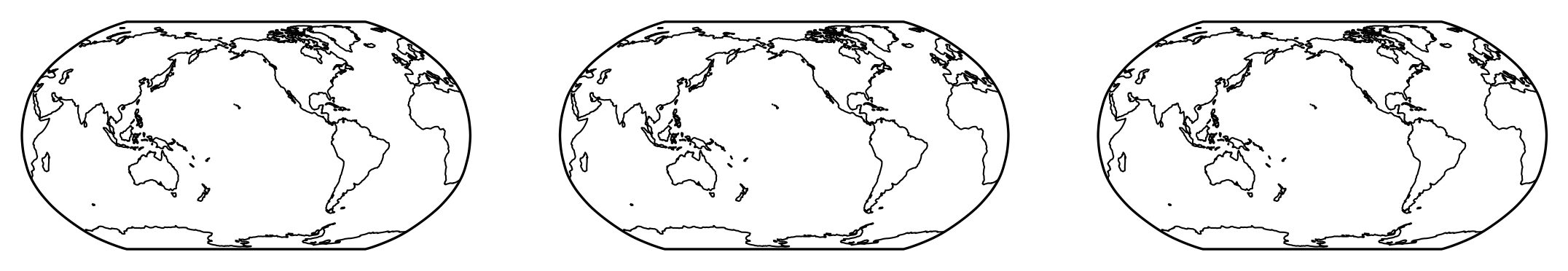
    season   <U3 12B 'JJA'

xarray.DataArray

• lat: 96
• lon: 144

• dask.array<chunksize=(96, 144), meta=np.ndarray>

  Array Chunk Bytes 108.00 kiB 108.00 kiB Shape (96, 144) (96, 144) Dask graph 1 chunks in 19 graph layers Data type float64 numpy.ndarray

• Coordinates: (3)
  • lat
    (lat)
    float64
    -90.0 -88.11 -86.21 ... 88.11 90.0

    long_name :

    latitude

    units :

    degrees_north

    array([-90.      , -88.105263, -86.210526, -84.315789, -82.421053, -80.526316,
           -78.631579, -76.736842, -74.842105, -72.947368, -71.052632, -69.157895,
           -67.263158, -65.368421, -63.473684, -61.578947, -59.684211, -57.789474,
           -55.894737, -54.      , -52.105263, -50.210526, -48.315789, -46.421053,
           -44.526316, -42.631579, -40.736842, -38.842105, -36.947368, -35.052632,
           -33.157895, -31.263158, -29.368421, -27.473684, -25.578947, -23.684211,
           -21.789474, -19.894737, -18.      , -16.105263, -14.210526, -12.315789,
           -10.421053,  -8.526316,  -6.631579,  -4.736842,  -2.842105,  -0.947368,
             0.947368,   2.842105,   4.736842,   6.631579,   8.526316,  10.421053,
            12.315789,  14.210526,  16.105263,  18.      ,  19.894737,  21.789474,
            23.684211,  25.578947,  27.473684,  29.368421,  31.263158,  33.157895,
            35.052632,  36.947368,  38.842105,  40.736842,  42.631579,  44.526316,
            46.421053,  48.315789,  50.210526,  52.105263,  54.      ,  55.894737,
            57.789474,  59.684211,  61.578947,  63.473684,  65.368421,  67.263158,
            69.157895,  71.052632,  72.947368,  74.842105,  76.736842,  78.631579,
            80.526316,  82.421053,  84.315789,  86.210526,  88.105263,  90.      ])

  • lon
    (lon)
    float64
    0.0 2.5 5.0 ... 352.5 355.0 357.5

    long_name :

    longitude

    units :

    degrees_east

    array([  0. ,   2.5,   5. ,   7.5,  10. ,  12.5,  15. ,  17.5,  20. ,  22.5,
            25. ,  27.5,  30. ,  32.5,  35. ,  37.5,  40. ,  42.5,  45. ,  47.5,
            50. ,  52.5,  55. ,  57.5,  60. ,  62.5,  65. ,  67.5,  70. ,  72.5,
            75. ,  77.5,  80. ,  82.5,  85. ,  87.5,  90. ,  92.5,  95. ,  97.5,
           100. , 102.5, 105. , 107.5, 110. , 112.5, 115. , 117.5, 120. , 122.5,
           125. , 127.5, 130. , 132.5, 135. , 137.5, 140. , 142.5, 145. , 147.5,
           150. , 152.5, 155. , 157.5, 160. , 162.5, 165. , 167.5, 170. , 172.5,
           175. , 177.5, 180. , 182.5, 185. , 187.5, 190. , 192.5, 195. , 197.5,
           200. , 202.5, 205. , 207.5, 210. , 212.5, 215. , 217.5, 220. , 222.5,
           225. , 227.5, 230. , 232.5, 235. , 237.5, 240. , 242.5, 245. , 247.5,
           250. , 252.5, 255. , 257.5, 260. , 262.5, 265. , 267.5, 270. , 272.5,
           275. , 277.5, 280. , 282.5, 285. , 287.5, 290. , 292.5, 295. , 297.5,
           300. , 302.5, 305. , 307.5, 310. , 312.5, 315. , 317.5, 320. , 322.5,
           325. , 327.5, 330. , 332.5, 335. , 337.5, 340. , 342.5, 345. , 347.5,
           350. , 352.5, 355. , 357.5])

  • season
    ()
    <U3
    'JJA'

    array('JJA', dtype='<U3')

• Indexes: (2)
  • lat
    PandasIndex

    PandasIndex(Index([              -90.0,  -88.10526315789474,  -86.21052631578948,
             -84.3157894736842,  -82.42105263157895,  -80.52631578947368,
            -78.63157894736842,  -76.73684210526316,  -74.84210526315789,
            -72.94736842105263,  -71.05263157894737,  -69.15789473684211,
            -67.26315789473685,  -65.36842105263158, -63.473684210526315,
           -61.578947368421055, -59.684210526315795,  -57.78947368421053,
            -55.89473684210527,               -54.0,  -52.10526315789474,
            -50.21052631578947,  -48.31578947368421,  -46.42105263157895,
           -44.526315789473685, -42.631578947368425,  -40.73684210526316,
             -38.8421052631579,  -36.94736842105264,  -35.05263157894737,
            -33.15789473684211, -31.263157894736842, -29.368421052631582,
           -27.473684210526322, -25.578947368421055, -23.684210526315795,
           -21.789473684210535,  -19.89473684210526,               -18.0,
            -16.10526315789474,  -14.21052631578948,  -12.31578947368422,
           -10.421052631578945,  -8.526315789473685,  -6.631578947368425,
            -4.736842105263165, -2.8421052631579045, -0.9473684210526301,
            0.9473684210526301,  2.8421052631578902,    4.73684210526315,
             6.631578947368411,   8.526315789473685,  10.421052631578945,
            12.315789473684205,  14.210526315789465,  16.105263157894726,
                          18.0,   19.89473684210526,   21.78947368421052,
             23.68421052631578,   25.57894736842104,  27.473684210526315,
            29.368421052631575,  31.263157894736835,  33.157894736842096,
            35.052631578947356,   36.94736842105263,   38.84210526315789,
             40.73684210526315,   42.63157894736841,   44.52631578947367,
             46.42105263157893,   48.31578947368419,   50.21052631578948,
             52.10526315789474,                54.0,   55.89473684210526,
             57.78947368421052,   59.68421052631578,   61.57894736842104,
              63.4736842105263,   65.36842105263156,   67.26315789473682,
             69.15789473684211,   71.05263157894737,   72.94736842105263,
             74.84210526315789,   76.73684210526315,   78.63157894736841,
             80.52631578947367,   82.42105263157893,   84.31578947368419,
             86.21052631578945,   88.10526315789474,                90.0],
          dtype='float64', name='lat'))

  • lon
    PandasIndex

    PandasIndex(Index([  0.0,   2.5,   5.0,   7.5,  10.0,  12.5,  15.0,  17.5,  20.0,  22.5,
           ...
           335.0, 337.5, 340.0, 342.5, 345.0, 347.5, 350.0, 352.5, 355.0, 357.5],
          dtype='float64', name='lon', length=144))

• Attributes: (0)

fig, axes = plt.subplots(1, 3, figsize=(9, 3), subplot_kw={
    'projection': ccrs.Robinson(central_longitude=210)})

# Use the first subplot for response to orbital forcing (PREC_MH - PREC_PI)
ax0 = axes[0]


# Use the second subplot for response to vegetation forcing (PREC_MHGS - PREC_MH)
ax1 = axes[1]



# Use the third subplot for response to combined forcings (PREC_MHGS - PREC_PI)
ax2 = axes[2]



for ax in axes:
    ax.coastlines(linewidth=0.5)

Click here for the solution

Copy and paste the code into the above cell

# Use the first subplot for response to orbital forcing
ax0 = axes[0]

prec_MH_ano = prec_MH_new - prec_PI_new

p0 = ax0.contourf(lon_new, prec_MH.lat, prec_MH_ano,
                 cmap='BrBG',
                 levels=np.linspace(-5, 5, 21),
                 extend='both',
                 transform=ccrs.PlateCarree())
plt.colorbar(p0, orientation='horizontal', pad=0.03)
ax0.set_title("ORB forced: MH - PI")


# Use the second subplot for response to vegetation forcing
ax1 = axes[1]

prec_MHGS_new, lon_new = add_cyclic_point(prec_MHGS, prec_MHGS.lon)
prec_MHGS_ano = prec_MHGS_new - prec_MH_new

p1 = ax1.contourf(lon_new, prec_MH.lat, prec_MHGS_ano,
                 cmap='BrBG',
                 levels=np.linspace(-5, 5, 21),
                 extend='both',
                 transform=ccrs.PlateCarree())
plt.colorbar(p1, orientation='horizontal', pad=0.03)
ax1.set_title("VEG forced: MHGS - MH")



# Use the third subplot for response to combined forcings
ax2 = axes[2]

prec_MHGS_ano2 = prec_MHGS_new - prec_PI_new

p2 = ax2.contourf(lon_new, prec_MH.lat, prec_MHGS_ano2,
                 cmap='BrBG',
                 levels=np.linspace(-5, 5, 21),
                 extend='both',
                 transform=ccrs.PlateCarree())
plt.colorbar(p2, orientation='horizontal', pad=0.03)
ax2.set_title("ORB + VEG forced: MHGS - PI")

Small group discussion

• How does the vegetation forcing over the Sahara impact the local precipitation?

• Does the vegetation forcing impact the ITCZ?

• Does the vegetation forcing impact the Walker Circulation?

• What do you see in the ORB-VEG combined response?

---

Summary so far

• We need longer simulations to allow the modeled climate state to reach equilibrium.

• Longer simulations also allows robust signal by removing internal variability.

• Both orbital and vegetation forcings impact atmosphere circulation, precipitation, and other climate states.

---

Optional

• Write your own code to explore the calendar effect by comparing files with and without cal_adj